Modeling Waves in Rivers and Canals

Note

This is a more advanced example that implements advanced channel hydraulics in RTC-Tools. It also capitalizes on the homotopy techniques available in RTC-Tools. If you are a first-time user of RTC-Tools, see Filling a Reservoir.

The RTC-Tools is capable of handling non-linear hydraulics. In this example, we model a river channel that receives a sudden pulse of higher-than-usual water volumes. We compare the results to those of an identical model built in HEC-RAS.

The Model

In this example, water is flowing through a single channel. There is an inflow at the upstream end and a water level bound at the downstream end.

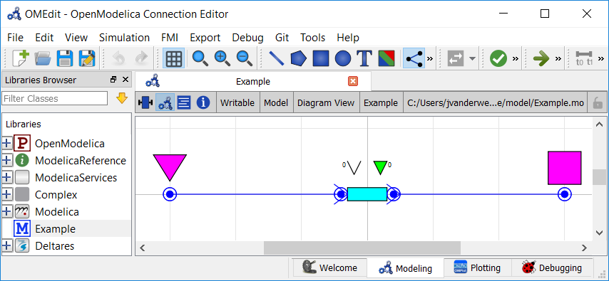
In OpenModelica Connection Editor, the model looks like this in plan view:

In text mode, the Modelica model looks as follows (with annotation statements removed):

model Example
  // Elements
  Deltares.ChannelFlow.Hydraulic.Branches.HomotopicTrapezoidal Channel(
    Q_nominal = 100.0,
    H_b_down = -5.0,
    H_b_up = -5.0,
    friction_coefficient = 0.045,
    use_manning = true,
    length = 10000,
    theta = theta,
    use_inertia = true,
    use_convective_acceleration = false,
    use_upwind = false,
    n_level_nodes = 11,
    uniform_nominal_depth = 5.0,
    bottom_width_down = 30,
    bottom_width_up = 30,
    left_slope_angle_up = 45,
    left_slope_angle_down = 45,
    right_slope_angle_up = 45,
    right_slope_angle_down = 45,
    semi_implicit_step_size = step_size
  ) ;
  Deltares.ChannelFlow.Hydraulic.BoundaryConditions.Level Level;
  Deltares.ChannelFlow.Hydraulic.BoundaryConditions.Discharge Discharge;
  // Inputs
  input Real Inflow_Q(fixed=true) = Discharge.Q;
  input Real Level_H(fixed=true) = Level.H;
  parameter Real theta;
  parameter Real step_size;
  // Output Channel states
  output Real Channel_Q_up = Discharge.Q;
  output Real Channel_Q_dn = Level.HQ.Q;
  output Real Channel_H_up = Discharge.HQ.H;
  output Real Channel_H_dn = Level.H;
equation
  connect(Channel.HQDown, Level.HQ);
  connect(Discharge.HQ, Channel.HQUp);
initial equation
  Channel.Q = fill(Inflow_Q, Channel.n_level_nodes + 1);
end Example;

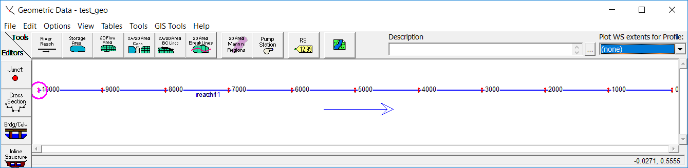
The plan view of the model looks like this in HEC-RAS:

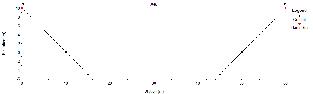
The channel cross-section is a simple trapezoidal shape. As rendered by HEC-RAS, here is a cross-section view of the channel being modeled:

The model was built with HEC-RAS version 5.0.6. In case you wish to verify the HEC-RAS model yourself, a zip of the HEC-RAS model used in this comparison is available: HEC-RAS.zip

The Python File

To keep this example simple and to allow for a 1:1 comparison with HEC-RAS, we will not have any decision variables in this model.

from rtctools.optimization.collocated_integrated_optimization_problem import (
    CollocatedIntegratedOptimizationProblem,
)
from rtctools.optimization.csv_mixin import CSVMixin
from rtctools.optimization.homotopy_mixin import HomotopyMixin
from rtctools.optimization.modelica_mixin import ModelicaMixin
from rtctools.util import run_optimization_problem


class Example(
    HomotopyMixin, CSVMixin, ModelicaMixin, CollocatedIntegratedOptimizationProblem
):
    def parameters(self, ensemble_member):
        p = super().parameters(ensemble_member)
        times = self.times()
        if self.use_semi_implicit:
            p['step_size'] = times[1] - times[0]
        else:
            p['step_size'] = 0.0
        p['Channel.use_convective_acceleration'] = self.use_convective_acceleration
        p['Channel.use_upwind'] = self.use_upwind
        return p

    def constraints(self, ensemble_member):
        constraints = super().constraints(ensemble_member)
        times = self.times()

        # Extract the number of nodes in the channel
        parameters = self.parameters(ensemble_member)
        n_level_nodes = int(parameters["Channel.n_level_nodes"])

        # To Mimic HEC-RAS behaviour, enforce steady state both at t0 and at t1.
        for i in range(n_level_nodes):
            state = "Channel.H[{}]".format(i + 1)
            constraints.append(
                (self.state_at(state, times[0]) - self.state_at(state, times[1]), 0, 0)
            )
        return constraints


class ExampleInertialWave(Example):
    """Inertial wave equation (no convective acceleration)"""

    model_name = 'Example'

    use_semi_implicit = False
    use_convective_acceleration = False
    use_upwind = False

    timeseries_export_basename = "timeseries_export_inertial_wave"


class ExampleInertialWaveSemiImplicit(Example):
    """Inertial wave equation (no convective acceleration)"""

    model_name = 'Example'

    use_semi_implicit = True
    use_convective_acceleration = False
    use_upwind = False

    timeseries_export_basename = "timeseries_export_inertial_wave_semi_implicit"


class ExampleSaintVenant(Example):
    """Saint Venant equation. Convective acceleration discretized with central differences"""

    model_name = 'Example'

    use_semi_implicit = False
    use_convective_acceleration = True
    use_upwind = False

    timeseries_export_basename = "timeseries_export_saint_venant"


class ExampleSaintVenantUpwind(Example):
    """Saint Venant equation. Convective acceleration discretized with upwind scheme"""

    model_name = 'Example'

    use_semi_implicit = False
    use_convective_acceleration = True
    use_upwind = True

    timeseries_export_basename = "timeseries_export_saint_venant_upwind"


run_optimization_problem(ExampleInertialWave)
run_optimization_problem(ExampleInertialWaveSemiImplicit)
run_optimization_problem(ExampleSaintVenant)
run_optimization_problem(ExampleSaintVenantUpwind)

As you can see, this model is as simple as it gets. We only add a constraint to keep the initialization states consistent with the HEC-RAS initialization.

Comparison of Discretizations and Numerical Schemes

HEC-RAS and RTC-Tools use different discretizations and numerical schemes, but also solve different equations. RTC-Tools solves the original nonlinear equations, whereas HEC-RAS solves a linearized momentum equation.

	RTC-Tools 2	HEC-RAS
Momentum equation	Saint-Venant / inertial wave (default)	Linearized Saint-Venant
Spatial discretization	Staggered	Collocated
Numerical scheme (temporal)	Semi-implicit / implicit (default)	Centered Preissmann box scheme
Numerical scheme (spatial)	Central differences, upwind convective acceleration (optional)	Centered Preissmann box scheme

Note

For optimization, the recommended momentum equation and temporal scheme for RTC-Tools is semi-implicit inertial wave. Consult Baayen and Piovesan, A continuation approach to nonlinear model predictive control of open channel systems, 2018, for details. A preprint is available online as arXiv:1801.06507.

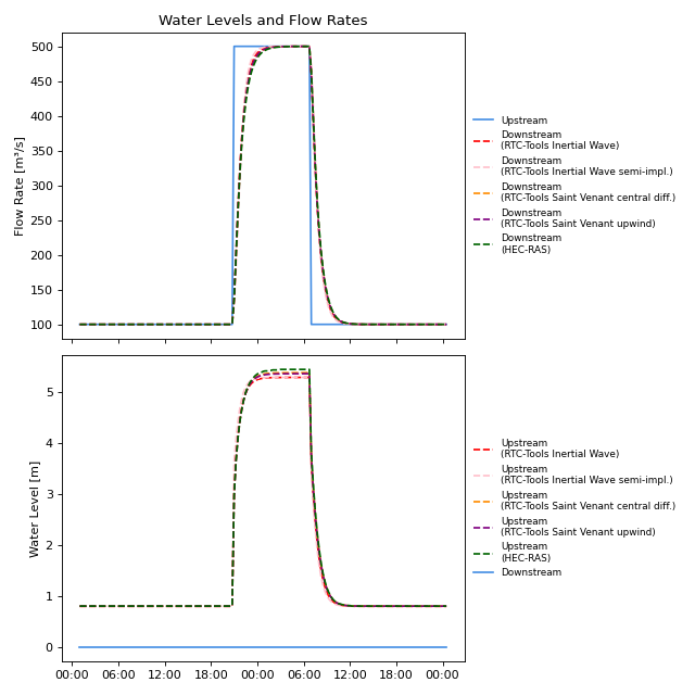
Comparison of Results

The results from the RTC-Tools run are found in the output directory with the name timeseries_export.csv, and the results generated by HEC-RAS have been exported into the same directory under the name HEC-RAS_results.csv. We can compare the results using the Python library matplotlib:

(Source code, svg, png)

Both HEC-RAS and RTC-Tools were run with a spatial step size of 1000 m and a temporal step size of 15 min.