Mixed Integer Optimization: Pumped Hydropower System (PHS)
Note
This example focuses on how to incorporate mixed integer components into a hydraulic model with an example in hydropower, and assumes basic exposure to RTC-Tools. To start with basics, see Filling a Reservoir.
Note
By default, if you define any integer or boolean variables in the model, RTC-Tools
will switch from IPOPT to BONMIN. You can modify solver options by overriding
the
solver_options()
method. Refer to CasADi’s nlpsol interface for a list of supported solvers. In this case we choose HiGHS
because the problem in a convex MIP and thus HiGHS can be used and tends to be faster than BONMIN.
The Model
For this example, the model represents a simpled Pumped Hydropower System.
The model can be viewed and edited using the OpenModelica Connection Editor
program. First load the Deltares library into OpenModelica Connection Editor,
and then load the example model, located at
<examples directory>\pumped_hydropower_system\model\PumpedStoragePlant.mo. The model PumpedStoragePlant.mo
represents a simple water system with the following elements:
an inflow boundary condition
Deltares.ChannelFlow.SimpleRouting.BoundaryConditions.Inflow,an upper reservoir modelled as a storage element
Deltares.ChannelFlow.SimpleRouting.Storage.Storage,an lower reservoir
Deltares.ChannelFlow.SimpleRouting.Reservoir.Reservoir,The PHS pump which pumps water from the lower to the upper reservoir
Deltares.ChannelFlow.SimpleRouting.Structures.DischargeControlledStructure,The PHS turbine which generates energy while water flows from the upper to lower reservoir
Deltares.ChannelFlow.SimpleRouting.Structures.DischargeControlledStructure,an outflow boundary condition
Deltares.ChannelFlow.SimpleRouting.BoundaryConditions.Terminal,

In text mode, the Modelica model looks as follows (with annotation statements removed):
 1model PumpedStoragePlant
 2  import SI = Modelica.Units.SI;
 3  // Declare Model Elements
 4  Deltares.ChannelFlow.SimpleRouting.BoundaryConditions.Inflow Inflow annotation(
 5    Placement(visible = true, transformation(origin = {-68, -4}, extent = {{-10, -10}, {10, 10}}, rotation = 0)));
 6  Deltares.ChannelFlow.SimpleRouting.BoundaryConditions.Terminal Outflow annotation(
 7    Placement(visible = true, transformation(origin = {80, -2}, extent = {{-10, -10}, {10, 10}}, rotation = 0)));
 8  Deltares.ChannelFlow.SimpleRouting.Storage.Storage UpperBasin annotation(
 9    Placement(visible = true, transformation(origin = {12, 82}, extent = {{-10, -10}, {10, 10}}, rotation = 0)));
10  Deltares.ChannelFlow.SimpleRouting.Reservoir.Reservoir LowerBasin(n_QLateral = 2) annotation(
11    Placement(visible = trued, transformation(origin = {-8, 6}, extent = {{-10, -10}, {10, 10}}, rotation = 0)));
12  Deltares.ChannelFlow.SimpleRouting.Structures.DischargeControlledStructure Pump annotation(
13    Placement(visible = true, transformation(origin = {-24, 56}, extent = {{-10, -10}, {10, 10}}, rotation = 90)));
14  Deltares.ChannelFlow.SimpleRouting.Structures.DischargeControlledStructure Turbine annotation(
15    Placement(visible = true, transformation(origin = {14, 46}, extent = {{-10, -10}, {10, 10}}, rotation = -90)));
16
17  // Define Input/Output Variables and set them equal to model variables
18  input SI.VolumeFlowRate Inflow_Q(fixed = true);
19  input SI.VolumeFlowRate PumpFlow(min = 0.0, max = 10.0, fixed = false);
20  input SI.VolumeFlowRate TurbineFlow(min = 0.0, max = 10.0, fixed = false);
21  input SI.VolumeFlowRate ReservoirTurbineFlow(min = 0.0, max = 100.0, fixed = false);
22  input SI.VolumeFlowRate ReservoirSpillFlow(min = 0.0, max = 100.0, fixed = false);
23  input Real cost_perP(fixed=true);
24  output Real PumpPower;
25  output Real TurbinePower;
26  output Real V_LowerBasin(min = 0.0, max = 1e7);
27  output Real V_UpperBasin(min = 0.0, max = 1e7);
28  output Real ReservoirPower;
29  output Real TotalSystemPower;
30  output Real TotalGeneratingPower(min = 0.0);
31  output Real SystemGeneratingRevenue;
32  output Real TotalSystemRevenue;
33  output Real TotalSystemRevenueSum;
34  output Real PumpCost;
35
36  // Define Boolean to ensure pumped storage turbine and pump cannot be used simultaneously
37  Boolean Turbine_is_on;
38
39  // Define constants for simple power calculations
40  parameter Real efficiency_reservoir = 0.88;
41  parameter Real efficiency_pump = 0.7;
42  parameter Real efficiency_turbine = 0.9;
43  parameter Real gravity = 9.81;
44  parameter Real rho = 1000.0;
45  parameter Real fix_dH_reservoir = 2.5;
46  parameter Real fix_dH_pump = 10.0;
47  parameter Real fix_dH_turbine = 10.0;
48
49equation
50  Inflow.QOut.Q = Inflow_Q;
51  Pump.Q = PumpFlow;
52  Turbine.Q = TurbineFlow;
53  LowerBasin.Q_turbine = ReservoirTurbineFlow;
54  LowerBasin.Q_spill = ReservoirSpillFlow;
55  V_LowerBasin = LowerBasin.V;
56  V_UpperBasin = UpperBasin.V;
57  PumpPower = efficiency_pump * PumpFlow * fix_dH_pump * gravity * rho;
58  TurbinePower = efficiency_turbine * TurbineFlow * fix_dH_turbine * gravity * rho;
59  ReservoirPower = efficiency_reservoir * gravity * rho * fix_dH_reservoir * ReservoirTurbineFlow;
60  TotalSystemPower = ReservoirPower + TurbinePower - PumpPower;
61  TotalGeneratingPower = ReservoirPower + TurbinePower;
62  PumpCost = PumpPower * cost_perP;
63  SystemGeneratingRevenue = TotalGeneratingPower*cost_perP;
64  TotalSystemRevenue = SystemGeneratingRevenue-PumpCost;
65  TotalSystemRevenueSum = transpose(sum(TotalSystemRevenue));
66
67  // Connect elements
68  connect(Turbine.QOut, LowerBasin.QLateral[2]) annotation(
69    Line(points = {{14, 38}, {-4, 38}, {-4, 14}}));
70  connect(Inflow.QOut, LowerBasin.QIn) annotation(
71    Line(points = {{-60, -4}, {-37, -4}, {-37, 6}, {-16, 6}}));
72  connect(LowerBasin.QOut, Outflow.QIn) annotation(
73    Line(points = {{0, 6}, {37, 6}, {37, -2}, {72, -2}}));
74  connect(LowerBasin.QLateral[1], Pump.QIn) annotation(
75    Line(points = {{-4, 14}, {-24, 14}, {-24, 48}}, thickness = 0.5));
76  connect(UpperBasin.QOut, Turbine.QIn) annotation(
77    Line(points = {{20, 82}, {14, 82}, {14, 54}}));
78  connect(Pump.QOut, UpperBasin.QIn) annotation(
79    Line(points = {{-24, 64}, {4, 64}, {4, 82}}));
80end PumpedStoragePlant;
The five water system elements (inflow boundary condition, storage, reservoir, Discharge
controlled structure and outflow boundary condition) appear under the model PumpedStoragePlant
statement. The equation part connects these five elements with the help of
connections.
In addition to elements, the input variables Inflow_Q, PumpFlow, TurbineFlow,
ReservoirTurbineFlow, ReservoirSpillFlow and cost_perP are also defined. Because
we want to view the power output and costs in the output file, we also define output
variables PumpPower, TurbinePower, V_LowerBasin,``V_UpperBasin``, ReservoirPower,
TotalSystemPower,``TotalGeneratingPower``, SystemGeneratingRevenue, TotalSystemRevenue,
TotalSystemRevenueSum, PumpCost.
To maintain represent the behaviour of a reversible PHS pump/turbine unit, we input the Boolean
Turbine_is_on as a way to ensure the PHS unit cannot be pumping and generating at the same time.
This variable is not used directly in the hydraulics, but we use it later in the
constraints in the python file.
The Optimization Problem
The python script consists of the following blocks:
Import of packages
Definition of goals
Definition of the optimization problem class
Pre-processing
Setting of varaible nominals
Definition of constraints
Additional configuration of the solver
Post-processing
A run statement
Importing Packages
For this example, the import block is as follows:
 1import numpy as np
 2
 3from rtctools.optimization.collocated_integrated_optimization_problem import (
 4    CollocatedIntegratedOptimizationProblem,
 5)
 6from rtctools.optimization.csv_mixin import CSVMixin
 7from rtctools.optimization.goal_programming_mixin import GoalProgrammingMixin, StateGoal
 8from rtctools.optimization.linearized_order_goal_programming_mixin import (
 9    LinearizedOrderGoalProgrammingMixin,
10)
11from rtctools.optimization.modelica_mixin import ModelicaMixin
12from rtctools.util import run_optimization_problem
Optimization Problem
First we define any goals we want to use during the optimization. These classes extend the Goal
class of RTC-Tools.
The TargetGoal calculates the deviations from the state and the target_min
and target_max. It is of order 4, so it then minimizes the sum of these deviations raised to the
power of 4. For this example the class is defined as follows.
15class TargetGoal(StateGoal):
16    order = 4
17
18    def __init__(
19        self,
20        optimization_problem,
21        state,
22        target_min,
23        target_max,
24        function_range,
25        priority,
26        function_nominal=1,
27    ):
28        self.state = state
29        self.target_min = target_min
30        self.target_max = target_max
31        self.priority = priority
32        super().__init__(optimization_problem)
33        self.function_range = function_range
34        self.function_nominal = function_nominal
The MaxRevenueGoal maximizes the state variable. To achieve this, we minimize the negative of the
state. For this example the class is defined as follows.
37class MaxRevenueGoal(StateGoal):
38    order = 1
39    state = "SystemGeneratingRevenue"
40    priority = 30
41
42    def function(self, optimization_problem, ensemble_member):
43        return -optimization_problem.state(self.state)
The MinCostGoal minimizes the state which is passed to the goal. For this example the class is
defined as follows.
46class MinCostGoal(StateGoal):
47    order = 1
48    state = "PumpCost"
49    priority = 25
Next, we construct the class by declaring it and inheriting the desired parent classes.
51
52class PumpStorage(
53    LinearizedOrderGoalProgrammingMixin,
54    GoalProgrammingMixin,
55    CSVMixin,
56    ModelicaMixin,
57    CollocatedIntegratedOptimizationProblem,
58):
59    model_name = "PumpedStoragePlant"
The pre-processing is called before any goals are added. Here we define a power_nominal.
This is the average of the Target_Power timeseries and is used to improve the scaling
of the model.
61    def pre(self):
62        super().pre()
63        self.power_nominal = np.mean(self.get_timeseries("Target_Power").values)
Constraints can be declared by the path_constraints() method.
Path constraints are constraints that are applied every timestep. To set a
constraint at an individual timestep, define it inside the constraints
method. Four constraints are added using the Big-M formulation to ensure the pumps and Turbine
joining the upper and lower reservoirs cannot be used at the same time.
65    def path_constraints(self, ensemble_member):
66        """
67        These constraints are formulated using the Big-M notation and represent the reversible
68        pump-turbine unit used to move water between the upper and lower reservoirs.
69
70        Boolean
71        -------
72        Turbine_is_on is a boolean which is 1 when the reversible unit is working as a turbine,
73        and 0 otherwsie. This is imposed by the following constraints
74
75        Constraints
76        -----------
77        0 <= PumpFlow + Turbine_is_on * M <= inf
78        0 <= TurbineFlow + (1 - Turbine_is_on) * M <= inf
79        -inf <= PumpFlow - (1 - Turbine_is_on) * M <= 0
80        -inf <= TurbineFlow - Turbine_is_on * M <= 0
81        """
82        constraints = super().path_constraints(ensemble_member)
83
84        M = 200.0
85        constraints.append((self.state("PumpFlow") + self.state("Turbine_is_on") * M, 0.0, np.inf))
86        constraints.append(
87            (self.state("TurbineFlow") + (1 - self.state("Turbine_is_on")) * M, 0.0, np.inf)
88        )
89        constraints.append(
90            (self.state("PumpFlow") - (1 - self.state("Turbine_is_on")) * M, -np.inf, 0.0)
91        )
92        constraints.append(
93            (self.state("TurbineFlow") - self.state("Turbine_is_on") * M, -np.inf, 0.0)
94        )
95
96        return constraints
Variable nominals can be set in the OpenModelica model file, or via the variable_nominal definition.
This can be useful when a variable nominal depends on a non-fixed value. Here the
power_nominal caluclated in the pre is set to be the nominal for the states TotalGeneratingPower
and TurbinePower.
 98    def variable_nominal(self, variable=None):
 99        nom = super().variable_nominal(variable)
100        if variable == "TotalGeneratingPower":
101            return self.power_nominal
102        elif variable == "TurbinePower":
103            return self.power_nominal
104        else:
105            return nom
The optimization objectives are added in path_goals. There are four goal in order of priority:
Priority 10
Goal to meet target power
Priority 20
Goal to minimize the spill of the lower reservoir
Priority 25
Minimize the cost associated with operating the pump
Priority 30
Maximize the revenue generated from using turbines at the upper and lower reservoir
107    def path_goals(self):
108        goals = super().path_goals()
109        # 020 goal to set the target spill flow as zero
110        goals.append(
111            TargetGoal(
112                self,
113                state="ReservoirSpillFlow",
114                target_min=np.nan,
115                target_max=0.0,
116                function_range=(0.0, 100.0),
117                priority=20,
118            )
119        )
120        # 030 goal to ensure the power generation meets the target
121        target = self.get_timeseries("Target_Power")
122        goals.append(
123            TargetGoal(
124                self,
125                state="TotalSystemPower",
126                target_min=target,
127                target_max=target,
128                function_range=(0.0, 4e6),
129                function_nominal=self.power_nominal,
130                priority=10,
131            )
132        )
133        # 040 goal to minimise the cost of the pump
134        goals.append(MinCostGoal(self))
135        # 050 goal to maximise the revenue from the turbines
136        goals.append(MaxRevenueGoal(self))
137
138        return goals
We want to apply some additional configuration, choosing the HiGHS solver over the default choice of bonmin for solving the mixed integer optimization problem. :
140    def solver_options(self):
141        options = super().solver_options()
142        options["casadi_solver"] = "qpsol"
143        options["solver"] = "highs"
144        return options
Finally, we want to print the Total revenue of the system. This can be done in the post.
146    def post(self):
147        super().post()
148        results = self.extract_results()
149        results["TotalSystemRevenueSum"] = np.sum(results["TotalSystemRevenue"])
150        print("Total Revenue is " + str(results["TotalSystemRevenueSum"]))
Run the Optimization Problem
To make our script run, at the bottom of our file we just have to call
the run_optimization_problem() method we imported on the optimization
problem class we just created.
154run_optimization_problem(PumpStorage)
The Whole Script
All together, the whole example script is as follows:
  1import numpy as np
  2
  3from rtctools.optimization.collocated_integrated_optimization_problem import (
  4    CollocatedIntegratedOptimizationProblem,
  5)
  6from rtctools.optimization.csv_mixin import CSVMixin
  7from rtctools.optimization.goal_programming_mixin import GoalProgrammingMixin, StateGoal
  8from rtctools.optimization.linearized_order_goal_programming_mixin import (
  9    LinearizedOrderGoalProgrammingMixin,
 10)
 11from rtctools.optimization.modelica_mixin import ModelicaMixin
 12from rtctools.util import run_optimization_problem
 13
 14
 15class TargetGoal(StateGoal):
 16    order = 4
 17
 18    def __init__(
 19        self,
 20        optimization_problem,
 21        state,
 22        target_min,
 23        target_max,
 24        function_range,
 25        priority,
 26        function_nominal=1,
 27    ):
 28        self.state = state
 29        self.target_min = target_min
 30        self.target_max = target_max
 31        self.priority = priority
 32        super().__init__(optimization_problem)
 33        self.function_range = function_range
 34        self.function_nominal = function_nominal
 35
 36
 37class MaxRevenueGoal(StateGoal):
 38    order = 1
 39    state = "SystemGeneratingRevenue"
 40    priority = 30
 41
 42    def function(self, optimization_problem, ensemble_member):
 43        return -optimization_problem.state(self.state)
 44
 45
 46class MinCostGoal(StateGoal):
 47    order = 1
 48    state = "PumpCost"
 49    priority = 25
 50
 51
 52class PumpStorage(
 53    LinearizedOrderGoalProgrammingMixin,
 54    GoalProgrammingMixin,
 55    CSVMixin,
 56    ModelicaMixin,
 57    CollocatedIntegratedOptimizationProblem,
 58):
 59    model_name = "PumpedStoragePlant"
 60
 61    def pre(self):
 62        super().pre()
 63        self.power_nominal = np.mean(self.get_timeseries("Target_Power").values)
 64
 65    def path_constraints(self, ensemble_member):
 66        """
 67        These constraints are formulated using the Big-M notation and represent the reversible
 68        pump-turbine unit used to move water between the upper and lower reservoirs.
 69
 70        Boolean
 71        -------
 72        Turbine_is_on is a boolean which is 1 when the reversible unit is working as a turbine,
 73        and 0 otherwsie. This is imposed by the following constraints
 74
 75        Constraints
 76        -----------
 77        0 <= PumpFlow + Turbine_is_on * M <= inf
 78        0 <= TurbineFlow + (1 - Turbine_is_on) * M <= inf
 79        -inf <= PumpFlow - (1 - Turbine_is_on) * M <= 0
 80        -inf <= TurbineFlow - Turbine_is_on * M <= 0
 81        """
 82        constraints = super().path_constraints(ensemble_member)
 83
 84        M = 200.0
 85        constraints.append((self.state("PumpFlow") + self.state("Turbine_is_on") * M, 0.0, np.inf))
 86        constraints.append(
 87            (self.state("TurbineFlow") + (1 - self.state("Turbine_is_on")) * M, 0.0, np.inf)
 88        )
 89        constraints.append(
 90            (self.state("PumpFlow") - (1 - self.state("Turbine_is_on")) * M, -np.inf, 0.0)
 91        )
 92        constraints.append(
 93            (self.state("TurbineFlow") - self.state("Turbine_is_on") * M, -np.inf, 0.0)
 94        )
 95
 96        return constraints
 97
 98    def variable_nominal(self, variable=None):
 99        nom = super().variable_nominal(variable)
100        if variable == "TotalGeneratingPower":
101            return self.power_nominal
102        elif variable == "TurbinePower":
103            return self.power_nominal
104        else:
105            return nom
106
107    def path_goals(self):
108        goals = super().path_goals()
109        # 020 goal to set the target spill flow as zero
110        goals.append(
111            TargetGoal(
112                self,
113                state="ReservoirSpillFlow",
114                target_min=np.nan,
115                target_max=0.0,
116                function_range=(0.0, 100.0),
117                priority=20,
118            )
119        )
120        # 030 goal to ensure the power generation meets the target
121        target = self.get_timeseries("Target_Power")
122        goals.append(
123            TargetGoal(
124                self,
125                state="TotalSystemPower",
126                target_min=target,
127                target_max=target,
128                function_range=(0.0, 4e6),
129                function_nominal=self.power_nominal,
130                priority=10,
131            )
132        )
133        # 040 goal to minimise the cost of the pump
134        goals.append(MinCostGoal(self))
135        # 050 goal to maximise the revenue from the turbines
136        goals.append(MaxRevenueGoal(self))
137
138        return goals
139
140    def solver_options(self):
141        options = super().solver_options()
142        options["casadi_solver"] = "qpsol"
143        options["solver"] = "highs"
144        return options
145
146    def post(self):
147        super().post()
148        results = self.extract_results()
149        results["TotalSystemRevenueSum"] = np.sum(results["TotalSystemRevenue"])
150        print("Total Revenue is " + str(results["TotalSystemRevenueSum"]))
151
152
153# Run
154run_optimization_problem(PumpStorage)
Running the Optimization Problem
To run the model, run the python file. /examples/pumped_hydropower_system/src/example.py.
Extracting Results
The results from the run are found in output/timeseries_export.csv. Any
CSV-reading software can import it, but this is how results can be plotted using
the python library matplotlib:
from datetime import datetime
import matplotlib.dates as mdates
import matplotlib.pyplot as plt
import numpy as np
# Import Data
data_path = "../../../examples/pumped_hydropower_system/reference_output/timeseries_export.csv"
import_data_path = "../../../examples/pumped_hydropower_system/input//timeseries_import.csv"
results = np.genfromtxt(
data_path, delimiter=",", encoding=None, dtype=None, names=True, case_sensitive="lower"
)
inputs = np.genfromtxt(
import_data_path, delimiter=",", encoding=None, dtype=None, names=True, case_sensitive="lower"
)
# Get times as datetime objects
times = [datetime.strptime(x, "%Y-%m-%d %H:%M:%S") for x in results["time"]]
# Generate Plot
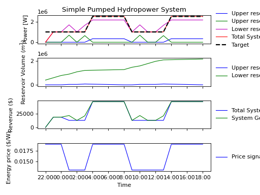
fig, axarr = plt.subplots(4, sharex=True)
axarr[0].set_title("Simple Pumped Hydropower System")
# Subplot 1
axarr[0].set_ylabel("Power [W]")
axarr[0].plot(
times, results["turbinepower"], label="Upper reservoir turbine", linewidth=1, color="b"
)
axarr[0].plot(times, results["pumppower"], label="Upper reservoir pumping", linewidth=1, color="g")
axarr[0].plot(
times, results["reservoirpower"], label="Lower reservoir turbine", linewidth=1, color="m"
)
axarr[0].plot(times, results["totalsystempower"], label="Total System", linewidth=1, color="r")
axarr[0].plot(
times,
inputs["target_power"],
label="Target",
linewidth=2,
color="black",
linestyle="--",
)
# Subplot 2
axarr[1].set_ylabel(r"Reservoir Volume ($m^3$)")
axarr[1].plot(times, results["v_upperbasin"], label="Upper reservoir", linewidth=1, color="b")
axarr[1].plot(times, results["v_lowerbasin"], label="Lower reservoir", linewidth=1, color="g")
# Subplot 3
axarr[2].set_ylabel(r"Revenue ($)")
axarr[2].plot(times, results["totalsystemrevenue"], label="Total System", linewidth=1, color="b")
axarr[2].plot(
times, results["systemgeneratingrevenue"], label="System Generating", linewidth=1, color="g"
)
# Subplot 4
axarr[3].set_ylabel(r"Energy price ($/W)")
axarr[3].plot(times, inputs["cost_perp"], label="Price signal", linewidth=1, color="b")
# Format bottom axis label
axarr[-1].xaxis.set_major_formatter(mdates.DateFormatter("%H:%M"))
axarr[-1].set_xlabel(r"Time")
# Shrink margins
fig.tight_layout()
# Shrink each axis and put a legend to the right of the axis
for i in range(len(axarr)):
box = axarr[i].get_position()
axarr[i].set_position([box.x0, box.y0, box.width * 0.8, box.height])
axarr[i].legend(loc="center left", bbox_to_anchor=(1, 0.5), frameon=False)
plt.autoscale(enable=True, axis="x", tight=True)
# Output Plot
plt.show()
(Source code, svg, png)

Observations
The target power is met and to do so, the upper reservoir (pumped storage) is used. As we want to minimize the cost of using the pump, the pump is used only when the cost is low.