Controlling a Cascade of Weirs: Local PID Control vs. Optimization
Note
This is a more advanced example that implements multi-objective optimization in RTC-Tools. It also capitalizes on the homotopy techniques available in RTC-Tools. If you are a first-time user of RTC-Tools, see Filling a Reservoir.
One of the advantages of using RTC-Tools for control is that it is capable of making decisions that are optimal for the whole network and for all future timesteps within the model time horizon. This is in contrast to local control algorithms such as PID controllers, where the control decision must be made on past states and local information alone. Furthermore, unlike a PID-style controller, RTC-Tools does not have gain parameters that need to be tuned.
This example models a cascading channel system, and compares a local control scheme using PID controllers with the RTC-Tools approach that uses Goal Programming.
The Model
For this example, water is flowing through a multilevel channel system. The model has three channel sections. There is an inflow forcing at the upstream boundary and a water level at the downstream boundary. The decision variables are the flow rates (and by extension, the weir settings) between the channels.
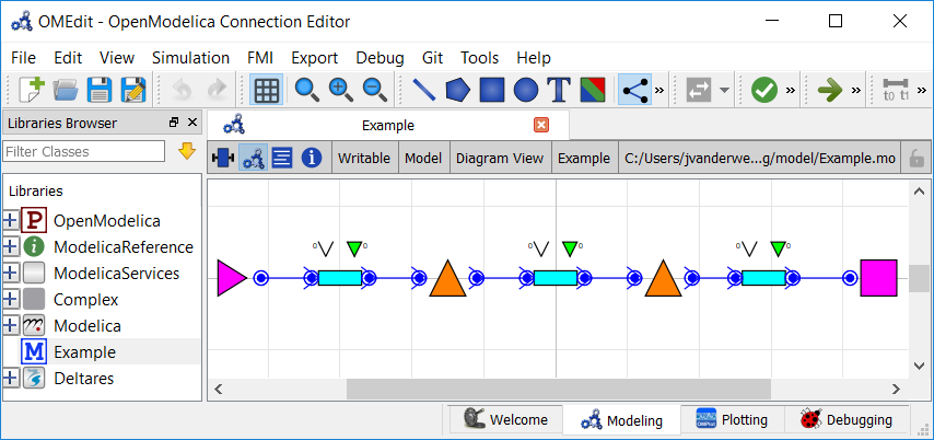
In OpenModelica Connection Editor, the model looks like this:
In text mode, the Modelica model looks as follows (with annotation statements removed):
 1model Example
 2  // Structures
 3  Deltares.ChannelFlow.Hydraulic.BoundaryConditions.Discharge Discharge;
 4  Deltares.ChannelFlow.Hydraulic.BoundaryConditions.Level Level;
 5  Deltares.ChannelFlow.Hydraulic.Branches.HomotopicTrapezoidal upstream(
 6    theta = theta,
 7    semi_implicit_step_size = step_size,
 8    H_b_up = 15,
 9    H_b_down = 15,
10    bottom_width_up = 50,
11    bottom_width_down = 50,
12    length = 20000,
13    uniform_nominal_depth = 5,
14    friction_coefficient = 35,
15    n_level_nodes = 4,
16    Q_nominal = 100.0
17  );
18  Deltares.ChannelFlow.Hydraulic.Branches.HomotopicTrapezoidal middle(
19    theta = theta,
20    semi_implicit_step_size = step_size,
21    H_b_up = 10,
22    H_b_down = 10,
23    bottom_width_up = 50,
24    bottom_width_down = 50,
25    length = 20000,
26    uniform_nominal_depth = 5,
27    friction_coefficient = 35,
28    n_level_nodes = 4,
29    Q_nominal = 100.0
30  );
31  Deltares.ChannelFlow.Hydraulic.Branches.HomotopicTrapezoidal downstream(
32    theta = theta,
33    semi_implicit_step_size = step_size,
34    H_b_up = 5,
35    H_b_down = 5,
36    bottom_width_up = 50,
37    bottom_width_down = 50,
38    length = 20000,
39    uniform_nominal_depth = 5,
40    friction_coefficient = 35,
41    n_level_nodes = 4,
42    Q_nominal = 100.0
43  );
44  Deltares.ChannelFlow.Hydraulic.Structures.DischargeControlledStructure dam_middle;
45  Deltares.ChannelFlow.Hydraulic.Structures.DischargeControlledStructure dam_upstream;
46
47  // Inputs
48  input Modelica.Units.SI.Position Level_H(fixed = true) = Level.H;
49  input Modelica.Units.SI.VolumeFlowRate Inflow_Q(fixed = true) = Discharge.Q;
50
51  // Outputs
52  output Modelica.Units.SI.Position H_middle = middle.H[middle.n_level_nodes];
53  output Modelica.Units.SI.Position H_upstream = upstream.H[upstream.n_level_nodes];
54  output Modelica.Units.SI.VolumeFlowRate Q_in = Inflow_Q;
55
56  // Parameters
57  parameter Modelica.Units.SI.Duration step_size;
58  parameter Real theta;
59equation
60  connect(dam_middle.HQDown, downstream.HQUp);
61  connect(dam_middle.HQUp, middle.HQDown);
62  connect(dam_upstream.HQDown, middle.HQUp);
63  connect(dam_upstream.HQUp, upstream.HQDown);
64  connect(Discharge.HQ, upstream.HQUp);
65  connect(Level.HQ, downstream.HQDown);
66initial equation
67  downstream.Q[2:downstream.n_level_nodes + 1] = Inflow_Q;
68  middle.Q[2:middle.n_level_nodes + 1] = Inflow_Q;
69  upstream.Q[2:upstream.n_level_nodes + 1] = Inflow_Q;
70end Example;
Note
In order to simulate and show how the PID controllers activate only once the incoming wave has propagated downstream, we will discretize the model in time with a resolution of 5 minutes. With our spatial resolution of 4 level nodes per 20 km reach, this produces a CFL number of approximately 0.4.
For optimization-based control, such a fine temporal resolution is not needed, as the system is able to look ahead and plan corrective measures ahead of time. In this case, CFL numbers of up to 1 or even higher are typically used.
Nevertheless, in order to present a consistent comparison, a 5 minute
time step is also used for the optimization example. It is easy to explore
the effect of the time step size on the optimization results by changing the
value of the step_size class variable.
To run the model with the local control scheme, we make a second model that constrains the flow rates to the weir settings as determined by local PID controller elements:
 1model ExampleLocalControl
 2  extends Example;
 3  // Add PID Controllers that apply local control
 4  PIDController upstream_pid(
 5    state = dam_upstream.HQUp.H,
 6    target_value = 20.0,
 7    P = -200.0,
 8    I = -0.01,
 9    D = 0.0,
10    feed_forward = 100.0,
11    control_action = dam_upstream.Q
12  );
13  PIDController middle_pid(
14    state = dam_middle.HQUp.H,
15    target_value = 15.0,
16    P = -200.0,
17    I = -0.01,
18    D = 0.0,
19    feed_forward = 100.0,
20    control_action = dam_middle.Q
21  );
22  output Modelica.Units.SI.VolumeFlowRate Q_dam_upstream = dam_upstream.Q;
23  output Modelica.Units.SI.VolumeFlowRate Q_dam_middle = dam_middle.Q;
24end ExampleLocalControl;
The local control model makes use of a PID controller class:
 1model PIDController
 2  input Real state;
 3  parameter Real target_value;
 4  parameter Real P = 1.0;
 5  parameter Real I = 0.0;
 6  parameter Real D = 0.0;
 7  parameter Real feed_forward = 0.0;
 8  output Real control_action;
 9  Real _error;
10  Real error_integral(nominal = 3600);
11equation
12  _error = target_value - state;
13  der(error_integral) = _error;
14  control_action = feed_forward + P * _error + I * error_integral + D * der(_error);
15initial equation
16  error_integral = 0.0;
17end PIDController;
Important
Modellers should take care to set proper values for the initial
derivatives, in order to avoid spurious waves at the start of the
optimization run. In this example we assume a steady state initial
condition, as indicated and enforced by the SteadyStateInitializationMixin
in the Python code.
The Optimization Problem
Goals
In this model, we define a TargetLevelGoal to find a requested target level:
15class TargetLevelGoal(Goal):
16    """Really Simple Target Level Goal"""
17
18    def __init__(self, state, target_level):
19        self.function_range = target_level - 5.0, target_level + 5.0
20        self.function_nominal = target_level
21        self.target_min = target_level
22        self.target_max = target_level
23        self.state = state
24
25    def function(self, optimization_problem, ensemble_member):
26        return optimization_problem.state(self.state)
27
28    priority = 1
We will later apply this goal to the upstream and middle channels.
You can read more about the components of goals in the documentation: Multi-objective optimization.
Optimization Problem
We construct the class by declaring it and inheriting the desired parent classes.
31class ExampleOptimization(
32    StepSizeParameterMixin,
33    SteadyStateInitializationMixin,
34    HomotopyMixin,
35    GoalProgrammingMixin,
36    CSVMixin,
37    ModelicaMixin,
38    CollocatedIntegratedOptimizationProblem,
39):
The StepSizeParameterMixin defines the step size parameter and sets the optimization
time steps, while the SteadyStateInitializationMixin constrains the initial
conditions to be steady-state.
Next, we instantiate the goals. There are two water level goals, applied at the upper and middle channels. The goals are very simple—they just target a specific water level.
42    def path_goals(self):
43        # Add water level goals
44        return [
45            TargetLevelGoal("dam_upstream.HQUp.H", 20.0),
46            TargetLevelGoal("dam_middle.HQUp.H", 15.0),
47        ]
We want to apply these goals to every timestep, so we use the path_goals()
method. This is a method that returns a list of the path goals we defined above.
Note that with path goals, each timestep is implemented as an independent goal—
if we cannot satisfy our min/max on time step A, it will not affect our desire
to satisfy the goal at time step B.
For comparison, we also define an optimization problem that uses a local control scheme. This example does not use any goals, as the flow rate is regulated by the PID Controller.
13class ExampleLocalControl(
14    StepSizeParameterMixin,
15    SteadyStateInitializationMixin,
16    HomotopyMixin,
17    CSVMixin,
18    ModelicaMixin,
19    CollocatedIntegratedOptimizationProblem,
20):
21    """Local Control Approach"""
22
23    timeseries_export_basename = "timeseries_export_local_control"
Run the Optimization Problem
To make our script run, at the bottom of our file we just have to call the
run_optimization_problem() method we imported on the optimization problem
classes we just created. We do this for both the local control model and the
goal programming model.
51run_optimization_problem(ExampleOptimization)
52run_optimization_problem(ExampleLocalControl)
The Whole Script
All together, all the scripts are as as follows:
step_size_parameter_mixin.py:
 1import numpy as np
 2
 3from rtctools.optimization.optimization_problem import OptimizationProblem
 4
 5
 6class StepSizeParameterMixin(OptimizationProblem):
 7    step_size = 5 * 60  # 5 minutes
 8
 9    def times(self, variable=None):
10        times = super().times(variable)
11        return np.arange(times[0], times[-1], self.step_size)
12
13    def parameters(self, ensemble_member):
14        p = super().parameters(ensemble_member)
15        p["step_size"] = self.step_size
16        return p
steady_state_initialization_mixin.py:
 1from rtctools.optimization.optimization_problem import OptimizationProblem
 2
 3
 4class SteadyStateInitializationMixin(OptimizationProblem):
 5    def constraints(self, ensemble_member):
 6        c = super().constraints(ensemble_member)
 7        times = self.times()
 8        parameters = self.parameters(ensemble_member)
 9        # Force steady-state initialization at t0 and at t1.
10        for reach in ["upstream", "middle", "downstream"]:
11            for i in range(int(parameters[f"{reach}.n_level_nodes"]) + 1):
12                state = f"{reach}.Q[{i + 1}]"
13                c.append((self.der_at(state, times[0]), 0, 0))
14        return c
example_local_control.py:
 1from steady_state_initialization_mixin import SteadyStateInitializationMixin
 2from step_size_parameter_mixin import StepSizeParameterMixin
 3
 4from rtctools.optimization.collocated_integrated_optimization_problem import (
 5    CollocatedIntegratedOptimizationProblem,
 6)
 7from rtctools.optimization.csv_mixin import CSVMixin
 8from rtctools.optimization.homotopy_mixin import HomotopyMixin
 9from rtctools.optimization.modelica_mixin import ModelicaMixin
10from rtctools.util import run_optimization_problem
11
12
13class ExampleLocalControl(
14    StepSizeParameterMixin,
15    SteadyStateInitializationMixin,
16    HomotopyMixin,
17    CSVMixin,
18    ModelicaMixin,
19    CollocatedIntegratedOptimizationProblem,
20):
21    """Local Control Approach"""
22
23    timeseries_export_basename = "timeseries_export_local_control"
24
25
26if __name__ == "__main__":
27    run_optimization_problem(ExampleLocalControl)
example_optimization.py:
 1from example_local_control import ExampleLocalControl
 2from steady_state_initialization_mixin import SteadyStateInitializationMixin
 3from step_size_parameter_mixin import StepSizeParameterMixin
 4
 5from rtctools.optimization.collocated_integrated_optimization_problem import (
 6    CollocatedIntegratedOptimizationProblem,
 7)
 8from rtctools.optimization.csv_mixin import CSVMixin
 9from rtctools.optimization.goal_programming_mixin import Goal, GoalProgrammingMixin
10from rtctools.optimization.homotopy_mixin import HomotopyMixin
11from rtctools.optimization.modelica_mixin import ModelicaMixin
12from rtctools.util import run_optimization_problem
13
14
15class TargetLevelGoal(Goal):
16    """Really Simple Target Level Goal"""
17
18    def __init__(self, state, target_level):
19        self.function_range = target_level - 5.0, target_level + 5.0
20        self.function_nominal = target_level
21        self.target_min = target_level
22        self.target_max = target_level
23        self.state = state
24
25    def function(self, optimization_problem, ensemble_member):
26        return optimization_problem.state(self.state)
27
28    priority = 1
29
30
31class ExampleOptimization(
32    StepSizeParameterMixin,
33    SteadyStateInitializationMixin,
34    HomotopyMixin,
35    GoalProgrammingMixin,
36    CSVMixin,
37    ModelicaMixin,
38    CollocatedIntegratedOptimizationProblem,
39):
40    """Goal Programming Approach"""
41
42    def path_goals(self):
43        # Add water level goals
44        return [
45            TargetLevelGoal("dam_upstream.HQUp.H", 20.0),
46            TargetLevelGoal("dam_middle.HQUp.H", 15.0),
47        ]
48
49
50# Run
51run_optimization_problem(ExampleOptimization)
52run_optimization_problem(ExampleLocalControl)
Extracting Results
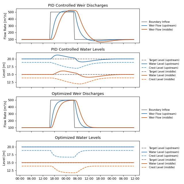
The results from the run are found in output/timeseries_export.csv and
output/timeseries_export_local_control.csv. Here are the results when
plotted using the python library matplotlib:
(Source code, svg, png)

In this example, the PID controller is tuned poorly and ends up amplifying the incoming wave as it propagates downstream. The optimizing controller, in contrast, does not amplify the wave and maintains the target water level throughout the wave event.