Goal Programming: Defining Multiple Objectives
Note
This example focuses on how to implement multi-objective optimization in RTC-Tools using Goal Programming. It assumes basic exposure to RTC-Tools. If you are a first-time user of RTC-Tools, see Filling a Reservoir.
Goal programming is a way to satisfy (sometimes conflicting) goals by ranking the goals by priority. The optimization algorithm will attempt to optimize each goal one at a time, starting with the goal with the highest priority and moving down through the list. Even if a goal cannot be satisfied, the goal programming algorithm will move on when it has found the best possible answer. Goals can be roughly divided into two types:
As long as we satisfy the goal, we do not care by how much. If we cannot satisfy a goal, any lower priority goals are not allowed to increase the amount by which we exceed (which is equivalent to not allowing any change at all to the exceedance).
We try to achieve as low a value as possible. Any lower priority goals are not allowed to result in an increase of this value (which is equivalent to not allowing any change at all).
In this example, we will be specifying two goals, on for each type. The higher priority goal will be to maintain the water level of the storage element between two levels. The lower priority goal will be to minimize the total volume pumped.
The Model
Note
This example uses the same hydraulic model as the MILP example. For a detailed explanation of the hydraulic model, including how to to formulate mixed integers in your model, see Mixed Integer Optimization: Pumps and Orifices.
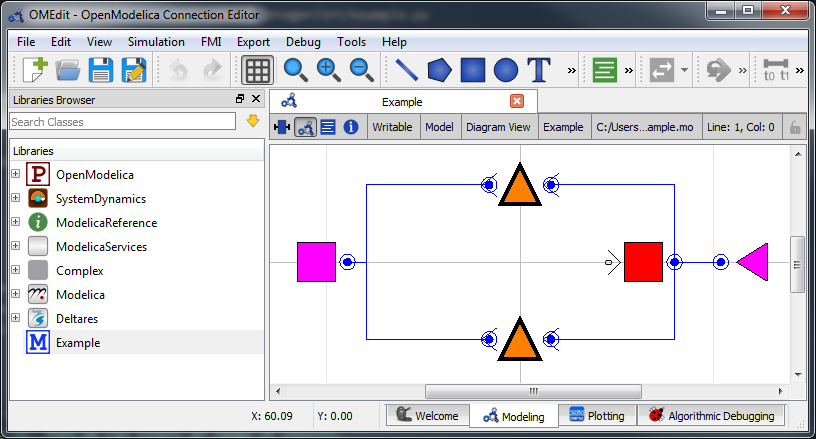
For this example, the model represents a typical setup for the dewatering of lowland areas. Water is routed from the hinterland (modeled as discharge boundary condition, right side) through a canal (modeled as storage element) towards the sea (modeled as water level boundary condition on the left side). Keeping the lowland area dry requires that enough water is discharged to the sea. If the sea water level is lower than the water level in the canal, the water can be discharged to the sea via gradient flow through the orifice (or a weir). If the sea water level is higher than in the canal, water must be pumped.
In OpenModelica Connection Editor, the model looks like this:
In text mode, the Modelica model looks as follows (with annotation statements removed):
 1model Example
 2  // Declare Model Elements
 3  Deltares.ChannelFlow.Hydraulic.Storage.Linear storage(A=1.0e6, H_b=0.0, HQ.H(min=0.0, max=0.5));
 4  Deltares.ChannelFlow.Hydraulic.BoundaryConditions.Discharge discharge;
 5  Deltares.ChannelFlow.Hydraulic.BoundaryConditions.Level level;
 6  Deltares.ChannelFlow.Hydraulic.Structures.Pump pump;
 7  Deltares.ChannelFlow.Hydraulic.Structures.Pump orifice;
 8
 9  // Define Input/Output Variables and set them equal to model variables
10  input Modelica.Units.SI.VolumeFlowRate Q_pump(fixed=false, min=0.0, max=7.0) = pump.Q;
11  input Boolean is_downhill;
12  input Modelica.Units.SI.VolumeFlowRate Q_in(fixed=true) = discharge.Q;
13  input Modelica.Units.SI.Position H_sea(fixed=true) = level.H;
14  input Modelica.Units.SI.VolumeFlowRate Q_orifice(fixed=false, min=0.0, max=10.0) = orifice.Q;
15  output Modelica.Units.SI.Position storage_level = storage.HQ.H;
16  output Modelica.Units.SI.Position sea_level = level.H;
17equation
18  // Connect Model Elements
19  connect(orifice.HQDown, level.HQ);
20  connect(storage.HQ, orifice.HQUp);
21  connect(storage.HQ, pump.HQUp);
22  connect(discharge.HQ, storage.HQ);
23  connect(pump.HQDown, level.HQ);
24end Example;
The Optimization Problem
When using goal programming, the python script consists of the following blocks:
Import of packages
Declaration of Goals
Declaration of the optimization problem class
Constructor
Declaration of constraint methods
Specification of Goals
Declaration of a
priority_completed()methodDeclaration of a
pre()methodDeclaration of a
post()methodAdditional configuration of the solver
A run statement
Importing Packages
For this example, the import block is as follows:
1import numpy as np
2
3from rtctools.optimization.collocated_integrated_optimization_problem import (
4    CollocatedIntegratedOptimizationProblem,
5)
6from rtctools.optimization.csv_mixin import CSVMixin
7from rtctools.optimization.goal_programming_mixin import Goal, GoalProgrammingMixin, StateGoal
8from rtctools.optimization.modelica_mixin import ModelicaMixin
Declaring Goals
Goals are defined as classes that inherit the Goal parent class. The
components of goals can be found in Multi-objective optimization. In
this example, we demonstrate three ways to define a goal in RTC-Tools.
First, we have a high priority goal to keep the water level within a minimum and
maximum. Since we are applying this goal to a specific state (model variable) in
our model at every time step, we can inherit a special helper class to define
this goal, called a StateGoal:
12class WaterLevelRangeGoal(StateGoal):
13    # Applying a state goal to every time step is easily done by defining a goal
14    # that inherits StateGoal. StateGoal is a helper class that uses the state
15    # to determine the function, function range, and function nominal
16    # automatically.
17    state = "storage.HQ.H"
18    # One goal can introduce a single or two constraints (min and/or max). Our
19    # target water level range is 0.43 - 0.44. We might not always be able to
20    # realize this, but we want to try.
21    target_min = 0.43
22    target_max = 0.44
23
24    # Because we want to satisfy our water level target first, this has a
25    # higher priority (=lower number).
26    priority = 1
We also want to save energy, so we define a goal to minimize the integral of
Q_pump. This goal has a lower priority than the water level range goal.
This goal does not use a helper class:
29class MinimizeQpumpGoal(Goal):
30    # This goal does not use a helper class, so we have to define the function
31    # method, range and nominal explicitly. We do not specify a target_min or
32    # target_max in this class, so the goal programming mixin will try to
33    # minimize the expression returned by the function method.
34    def function(self, optimization_problem, ensemble_member):
35        return optimization_problem.integral("Q_pump")
36
37    # The nominal is used to scale the value returned by
38    # the function method so that the value is on the order of 1.
39    function_nominal = 100.0
40    # The lower the number returned by this function, the higher the priority.
41    priority = 2
42    # The penalty variable is taken to the order'th power.
43    order = 1
We add a third goal minimizing the changes in``Q_pump``, and give it the least priority. This goal smooths out the operation of the pump so that it changes state as few times as possible. To get an idea of what the pump would have done without this goal, see Mixed Integer: Observations. The order of this goal must be 2, so that it penalizes both positive and negative derivatives. Order of 2 is the default, but we include it here explicitly for the sake of clarity.
46class MinimizeChangeInQpumpGoal(Goal):
47    # To reduce pump power cycles, we add a third goal to minimize changes in
48    # Q_pump. This will be passed into the optimization problem as a path goal
49    # because it is an an individual goal that should be applied at every time
50    # step.
51    def function(self, optimization_problem, ensemble_member):
52        return optimization_problem.der("Q_pump")
53
54    function_nominal = 5.0
55    priority = 3
56    # Default order is 2, but we want to be explicit
57    order = 2
Optimization Problem
Next, we construct the class by declaring it and inheriting the desired parent classes.
60class Example(
61    GoalProgrammingMixin, CSVMixin, ModelicaMixin, CollocatedIntegratedOptimizationProblem
62):
Constraints can be declared by declaring the path_constraints() method.
Path constraints are constraints that are applied every timestep. To set a
constraint at an individual timestep, define it inside the constraints()
method.
The “orifice” requires special constraints to be set in order to work. They are
implemented below in the path_constraints() method. Other parent classes
also declare this method, so we call the super() method so that we don’t
overwrite their behaviour.
 67    def path_constraints(self, ensemble_member):
 68        # We want to add a few hard constraints to our problem. The goal
 69        # programming mixin however also generates constraints (and objectives)
 70        # from on our goals, so we have to call super() here.
 71        constraints = super().path_constraints(ensemble_member)
 72
 73        # Release through orifice downhill only. This constraint enforces the
 74        # fact that water only flows downhill
 75        constraints.append(
 76            (self.state("Q_orifice") + (1 - self.state("is_downhill")) * 10, 0.0, 10.0)
 77        )
 78
 79        # Make sure is_downhill is true only when the sea is lower than the
 80        # water level in the storage.
 81        M = 2  # The so-called "big-M"
 82        constraints.append(
 83            (
 84                self.state("H_sea")
 85                - self.state("storage.HQ.H")
 86                - (1 - self.state("is_downhill")) * M,
 87                -np.inf,
 88                0.0,
 89            )
 90        )
 91        constraints.append(
 92            (
 93                self.state("H_sea") - self.state("storage.HQ.H") + self.state("is_downhill") * M,
 94                0.0,
 95                np.inf,
 96            )
 97        )
 98
 99        # Orifice flow constraint. Uses the equation:
100        # Q(HUp, HDown, d) = width * C * d * (2 * g * (HUp - HDown)) ^ 0.5
101        # Note that this equation is only valid for orifices that are submerged
102        #          units:  description:
103        w = 3.0  # m       width of orifice
104        d = 0.8  # m       hight of orifice
105        C = 1.0  # none    orifice constant
106        g = 9.8  # m/s^2   gravitational acceleration
107        constraints.append(
108            (
109                ((self.state("Q_orifice") / (w * C * d)) ** 2) / (2 * g)
110                + self.state("orifice.HQDown.H")
111                - self.state("orifice.HQUp.H")
112                - M * (1 - self.state("is_downhill")),
113                -np.inf,
114                0.0,
115            )
116        )
117
118        return constraints
Now we pass in the goals. There are path goals and normal goals, so we have to pass them in using separate methods. A path goal is a specific kind of goal that applies to a particular variable at an individual time step, but that we want to set for all the timesteps.
Non-path goals are more general goals that are not iteratively applied at every
timestep. We use the goals() method to pass a list of these goals to the
optimizer.
120    def goals(self):
121        return [MinimizeQpumpGoal()]
For the goals that want to apply our goals to every timestep, so we use the
path_goals() method. This is a method that returns a list of the path goals
we defined above. Note that with path goals, each timestep is implemented as an
independant goal- if we cannot satisfy our min/max on time step A, it will not
affect our desire to satisfy the goal at time step B. Goals that inherit
StateGoal are always path goals and must always be initialized with the
parameter self.
123    def path_goals(self):
124        # Sorting goals on priority is done in the goal programming mixin. We
125        # do not have to worry about order here.
126        return [WaterLevelRangeGoal(self), MinimizeChangeInQpumpGoal()]
If all we cared about were the results, we could end our class declaration here. However, it is usually helpful to track how the solution changes after optimizing each priority level. To track these changes, we need to add three methods.
The method pre() is already defined in RTC-Tools, but we would like to add
a line to it to create a variable for storing intermediate results. To do this,
we declare a new pre() method, call super().pre() to ensure
that the original method runs unmodified, and add in a variable declaration to
store our list of intermediate results:
128    def pre(self):
129        # Call super() class to not overwrite default behaviour
130        super().pre()
131        # We keep track of our intermediate results, so that we can print some
132        # information about the progress of goals at the end of our run.
133        self.intermediate_results = []
Next, we define the priority_completed() method to inspect and summarize the
results. These are appended to our intermediate results variable after each
priority is completed.
135    def priority_completed(self, priority):
136        # We want to show that the results of our highest priority goal (water
137        # level) are remembered. The other information we want to see is how our
138        # lower priority goal (Q_pump) progresses. We can write some code that
139        # sumerizes the results and stores it.
140
141        # A little bit of tolerance when checking for acceptance, because
142        # strictly speaking 0.4299... is smaller than 0.43.
143        _min = 0.43 - 1e-4
144        _max = 0.44 + 1e-4
145
146        results = self.extract_results()
147        n_level_satisfied = sum(1 for x in results["storage.HQ.H"] if _min <= x <= _max)
148        q_pump_integral = sum(results["Q_pump"])
149        q_pump_sum_changes = np.sum(np.diff(results["Q_pump"]) ** 2)
150        self.intermediate_results.append(
151            (priority, n_level_satisfied, q_pump_integral, q_pump_sum_changes)
152        )
We want some way to output our intermediate results. This is accomplished using
the post() method. Again, we nedd to call the super() method to avoid
overwiting the internal method.
154    def post(self):
155        # Call super() class to not overwrite default behaviour
156        super().post()
157        for (
158            priority,
159            n_level_satisfied,
160            q_pump_integral,
161            q_pump_sum_changes,
162        ) in self.intermediate_results:
163            print("\nAfter finishing goals of priority {}:".format(priority))
164            print(
165                "Level goal satisfied at {} of {} time steps".format(
166                    n_level_satisfied, len(self.times())
167                )
168            )
169            print("Integral of Q_pump = {:.2f}".format(q_pump_integral))
170            print("Sum of squares of changes in Q_pump: {:.2f}".format(q_pump_sum_changes))
Finally, we want to apply some additional configuration, reducing the amount of information the solver outputs:
173    def solver_options(self):
174        options = super().solver_options()
175        solver = options["solver"]
176        options[solver]["print_level"] = 1
177        return options
Run the Optimization Problem
To make our script run, at the bottom of our file we just have to call
the run_optimization_problem() method we imported on the optimization
problem class we just created.
181run_optimization_problem(Example)
The Whole Script
All together, the whole example script is as follows:
  1import numpy as np
  2
  3from rtctools.optimization.collocated_integrated_optimization_problem import (
  4    CollocatedIntegratedOptimizationProblem,
  5)
  6from rtctools.optimization.csv_mixin import CSVMixin
  7from rtctools.optimization.goal_programming_mixin import Goal, GoalProgrammingMixin, StateGoal
  8from rtctools.optimization.modelica_mixin import ModelicaMixin
  9from rtctools.util import run_optimization_problem
 10
 11
 12class WaterLevelRangeGoal(StateGoal):
 13    # Applying a state goal to every time step is easily done by defining a goal
 14    # that inherits StateGoal. StateGoal is a helper class that uses the state
 15    # to determine the function, function range, and function nominal
 16    # automatically.
 17    state = "storage.HQ.H"
 18    # One goal can introduce a single or two constraints (min and/or max). Our
 19    # target water level range is 0.43 - 0.44. We might not always be able to
 20    # realize this, but we want to try.
 21    target_min = 0.43
 22    target_max = 0.44
 23
 24    # Because we want to satisfy our water level target first, this has a
 25    # higher priority (=lower number).
 26    priority = 1
 27
 28
 29class MinimizeQpumpGoal(Goal):
 30    # This goal does not use a helper class, so we have to define the function
 31    # method, range and nominal explicitly. We do not specify a target_min or
 32    # target_max in this class, so the goal programming mixin will try to
 33    # minimize the expression returned by the function method.
 34    def function(self, optimization_problem, ensemble_member):
 35        return optimization_problem.integral("Q_pump")
 36
 37    # The nominal is used to scale the value returned by
 38    # the function method so that the value is on the order of 1.
 39    function_nominal = 100.0
 40    # The lower the number returned by this function, the higher the priority.
 41    priority = 2
 42    # The penalty variable is taken to the order'th power.
 43    order = 1
 44
 45
 46class MinimizeChangeInQpumpGoal(Goal):
 47    # To reduce pump power cycles, we add a third goal to minimize changes in
 48    # Q_pump. This will be passed into the optimization problem as a path goal
 49    # because it is an an individual goal that should be applied at every time
 50    # step.
 51    def function(self, optimization_problem, ensemble_member):
 52        return optimization_problem.der("Q_pump")
 53
 54    function_nominal = 5.0
 55    priority = 3
 56    # Default order is 2, but we want to be explicit
 57    order = 2
 58
 59
 60class Example(
 61    GoalProgrammingMixin, CSVMixin, ModelicaMixin, CollocatedIntegratedOptimizationProblem
 62):
 63    """
 64    An introductory example to goal programming in RTC-Tools
 65    """
 66
 67    def path_constraints(self, ensemble_member):
 68        # We want to add a few hard constraints to our problem. The goal
 69        # programming mixin however also generates constraints (and objectives)
 70        # from on our goals, so we have to call super() here.
 71        constraints = super().path_constraints(ensemble_member)
 72
 73        # Release through orifice downhill only. This constraint enforces the
 74        # fact that water only flows downhill
 75        constraints.append(
 76            (self.state("Q_orifice") + (1 - self.state("is_downhill")) * 10, 0.0, 10.0)
 77        )
 78
 79        # Make sure is_downhill is true only when the sea is lower than the
 80        # water level in the storage.
 81        M = 2  # The so-called "big-M"
 82        constraints.append(
 83            (
 84                self.state("H_sea")
 85                - self.state("storage.HQ.H")
 86                - (1 - self.state("is_downhill")) * M,
 87                -np.inf,
 88                0.0,
 89            )
 90        )
 91        constraints.append(
 92            (
 93                self.state("H_sea") - self.state("storage.HQ.H") + self.state("is_downhill") * M,
 94                0.0,
 95                np.inf,
 96            )
 97        )
 98
 99        # Orifice flow constraint. Uses the equation:
100        # Q(HUp, HDown, d) = width * C * d * (2 * g * (HUp - HDown)) ^ 0.5
101        # Note that this equation is only valid for orifices that are submerged
102        #          units:  description:
103        w = 3.0  # m       width of orifice
104        d = 0.8  # m       hight of orifice
105        C = 1.0  # none    orifice constant
106        g = 9.8  # m/s^2   gravitational acceleration
107        constraints.append(
108            (
109                ((self.state("Q_orifice") / (w * C * d)) ** 2) / (2 * g)
110                + self.state("orifice.HQDown.H")
111                - self.state("orifice.HQUp.H")
112                - M * (1 - self.state("is_downhill")),
113                -np.inf,
114                0.0,
115            )
116        )
117
118        return constraints
119
120    def goals(self):
121        return [MinimizeQpumpGoal()]
122
123    def path_goals(self):
124        # Sorting goals on priority is done in the goal programming mixin. We
125        # do not have to worry about order here.
126        return [WaterLevelRangeGoal(self), MinimizeChangeInQpumpGoal()]
127
128    def pre(self):
129        # Call super() class to not overwrite default behaviour
130        super().pre()
131        # We keep track of our intermediate results, so that we can print some
132        # information about the progress of goals at the end of our run.
133        self.intermediate_results = []
134
135    def priority_completed(self, priority):
136        # We want to show that the results of our highest priority goal (water
137        # level) are remembered. The other information we want to see is how our
138        # lower priority goal (Q_pump) progresses. We can write some code that
139        # sumerizes the results and stores it.
140
141        # A little bit of tolerance when checking for acceptance, because
142        # strictly speaking 0.4299... is smaller than 0.43.
143        _min = 0.43 - 1e-4
144        _max = 0.44 + 1e-4
145
146        results = self.extract_results()
147        n_level_satisfied = sum(1 for x in results["storage.HQ.H"] if _min <= x <= _max)
148        q_pump_integral = sum(results["Q_pump"])
149        q_pump_sum_changes = np.sum(np.diff(results["Q_pump"]) ** 2)
150        self.intermediate_results.append(
151            (priority, n_level_satisfied, q_pump_integral, q_pump_sum_changes)
152        )
153
154    def post(self):
155        # Call super() class to not overwrite default behaviour
156        super().post()
157        for (
158            priority,
159            n_level_satisfied,
160            q_pump_integral,
161            q_pump_sum_changes,
162        ) in self.intermediate_results:
163            print("\nAfter finishing goals of priority {}:".format(priority))
164            print(
165                "Level goal satisfied at {} of {} time steps".format(
166                    n_level_satisfied, len(self.times())
167                )
168            )
169            print("Integral of Q_pump = {:.2f}".format(q_pump_integral))
170            print("Sum of squares of changes in Q_pump: {:.2f}".format(q_pump_sum_changes))
171
172    # Any solver options can be set here
173    def solver_options(self):
174        options = super().solver_options()
175        solver = options["solver"]
176        options[solver]["print_level"] = 1
177        return options
178
179
180# Run
181run_optimization_problem(Example)
Running the Optimization Problem
Following the execution of the optimization problem, the post() method
should print out the following lines:
After finishing goals of priority 1:
Level goal satisfied at 19 of 21 time steps
Integral of Q_pump = 74.18
Sum of Changes in Q_pump: 7.83

After finishing goals of priority 2:
Level goal satisfied at 19 of 21 time steps
Integral of Q_pump = 60.10
Sum of Changes in Q_pump: 11.70

After finishing goals of priority 3:
Level goal satisfied at 19 of 21 time steps
Integral of Q_pump = 60.10
Sum of Changes in Q_pump: 10.07
As the output indicates, while optimizing for the priority 1 goal, no attempt
was made to minimize the integral of Q_pump. The only objective was to
minimize the number of states in violation of the water level goal.
After optimizing for the priority 2 goal, the solver was able to find a solution
that reduced the integral of Q_pump without increasing the number of
timesteps where the water level exceeded the limit. However, this solution
induced additional variation into the operation of Q_pump
After optimizing the priority 3 goal, the integral of Q_pump is the same and
the level goal has not improved. Without hurting any higher priority goals,
RTC-Tools was able to smooth out the operation of the pump.
Extracting Results
The results from the run are found in output/timeseries_export.csv. Any
CSV-reading software can import it, but this is how results can be plotted using
the python library matplotlib:
from datetime import datetime

import matplotlib.dates as mdates
import matplotlib.pyplot as plt
import numpy as np

# Import Data
data_path = "../../../examples/goal_programming/reference_output/timeseries_export.csv"
results = np.genfromtxt(
    data_path, delimiter=",", encoding=None, dtype=None, names=True, case_sensitive="lower"
)

# Get times as datetime objects
times = [datetime.strptime(x, "%Y-%m-%d %H:%M:%S") for x in results["time"]]

# Generate Plot
n_subplots = 3
fig, axarr = plt.subplots(n_subplots, sharex=True, figsize=(8, 3 * n_subplots))
axarr[0].set_title("Water Level and Discharge")

# Upper subplot
axarr[0].set_ylabel("Water Level [m]")
axarr[0].plot(times, results["storage_level"], label="Storage", linewidth=2, color="b")
axarr[0].plot(times, results["sea_level"], label="Sea", linewidth=2, color="m")

# Middle subplot
axarr[1].set_ylabel("Water Level [m]")
axarr[1].plot(times, results["storage_level"], label="Storage", linewidth=2, color="b")
axarr[1].plot(
    times,
    0.44 * np.ones_like(times),
    label="Storage Max",
    linewidth=2,
    color="r",
    linestyle="--",
)
axarr[1].plot(
    times,
    0.43 * np.ones_like(times),
    label="Storage Min",
    linewidth=2,
    color="g",
    linestyle="--",
)

# Lower Subplot
axarr[2].set_ylabel("Flow Rate [m³/s]")
axarr[2].scatter(times, results["q_orifice"], linewidth=1, color="g")
axarr[2].scatter(times, results["q_pump"], linewidth=1, color="r")
# add horizontal lines to the left of these dots, to indicate that the value is attained over an
# entire timestep:
axarr[2].step(times, results["q_orifice"], linewidth=2, where="pre", label="Orifice", color="g")
axarr[2].step(times, results["q_pump"], linewidth=1, where="pre", label="Pump", color="r")

# Format bottom axis label
axarr[-1].xaxis.set_major_formatter(mdates.DateFormatter("%H:%M"))

# Shrink margins
fig.tight_layout()

# Shrink each axis and put a legend to the right of the axis
for i in range(n_subplots):
    box = axarr[i].get_position()
    axarr[i].set_position([box.x0, box.y0, box.width * 0.8, box.height])
    axarr[i].legend(loc="center left", bbox_to_anchor=(1, 0.5), frameon=False)

plt.autoscale(enable=True, axis="x", tight=True)

# Output Plot
plt.show()
(Source code, svg, png)
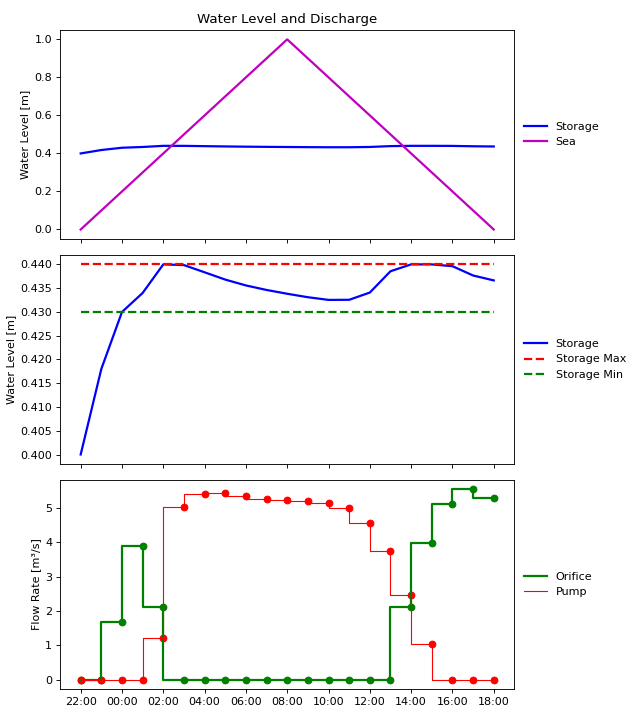

Observe that the red pump curve is indeed more smooth than what we have seen before. You may compare this picture with the one in the previous example (Mixed Integer Optimization). The observant user may conclude that although the curve is indeed more smooth, the surface area under the red curve also seems to have increased (i.e., in total, more water is pumped!) This is due to the extra goal that we introduced: the WaterLevelRangeGoal that wasn’t present in the Mixed Integer example. Experiment with commenting out this goal on line 109 to see how it affects the results.