Using Delay Equations

RTC-Tools supports using delay equations. This works for both optimization and simulation problems, although for simulation, this currently only works for a constant delay time and a constant timestep size.

To illustrate the use of delay equations, we consider the following integrator-delay model.

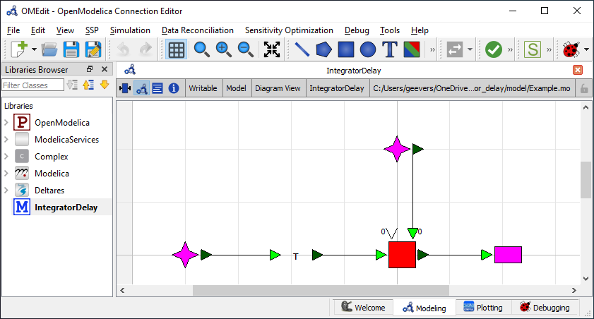
model Example
  parameter Integer delay_hours = 24.0;
  Deltares.ChannelFlow.SimpleRouting.BoundaryConditions.Inflow control_inflow annotation(
    Placement(visible = true, transformation(origin = {-80, 0}, extent = {{-10, -10}, {10, 10}}, rotation = 0)));
  Deltares.ChannelFlow.SimpleRouting.BoundaryConditions.Inflow external_inflow annotation(
    Placement(visible = true, transformation(origin = {0, 40}, extent = {{-10, -10}, {10, 10}}, rotation = 0)));
  Deltares.ChannelFlow.SimpleRouting.Branches.Delay delay_component(duration = delay_hours * 3600) annotation(
    Placement(visible = true, transformation(origin = {-38, 0}, extent = {{-10, -10}, {10, 10}}, rotation = 0)));
  Deltares.ChannelFlow.SimpleRouting.Branches.Integrator integrator(n_QLateral = 1) annotation(
    Placement(visible = true, transformation(origin = {2, 0}, extent = {{-10, -10}, {10, 10}}, rotation = 0)));
  Deltares.ChannelFlow.SimpleRouting.BoundaryConditions.Terminal outflow annotation(
    Placement(visible = true, transformation(origin = {42, 0}, extent = {{-10, -10}, {10, 10}}, rotation = 0)));
  input Modelica.SIunits.VolumeFlowRate Q_in(fixed = true);
  input Modelica.SIunits.VolumeFlowRate Q_out(fixed = true);
  input Modelica.SIunits.VolumeFlowRate Q_control(fixed = false);
  output Modelica.SIunits.Volume V_integrator;
equation
  // connect(control_inflow.QOut, integrator.QIn);
  connect(control_inflow.QOut, delay_component.QIn) annotation(
    Line(points = {{-72, 0}, {-46, 0}}));
  connect(delay_component.QOut, integrator.QIn) annotation(
    Line(points = {{-30, 0}, {-6, 0}}));
  connect(external_inflow.QOut, integrator.QLateral[1]) annotation(
    Line(points = {{8, 40}, {6, 40}, {6, 8}}));
  connect(integrator.QOut, outflow.QIn) annotation(
    Line(points = {{10, 0}, {34, 0}}));
  Q_control = control_inflow.Q;
  Q_in = external_inflow.Q;
  Q_out = outflow.Q;
  V_integrator = integrator.V;
end Example;

This model describes two inflows that come together. One of the inflows can be controlled and has a delay of 24 hours before joining the other inflow.

For the optimization problem, the goal is to keep the volume at a constant level of 400,000 cubic meter. The problem is given below.

class ExampleOpt(CSVMixinOpt, ModelicaMixin, CollocatedIntegratedOptimizationProblem):
    """
    An optimization problem example containing a delay component
    """

    def __init__(self, **kwargs):
        super().__init__(model_name="Example", **kwargs)

    def path_objective(self, ensemble_member):
        # The goal is that the volume stays as close to v_ideal as possible.
        del ensemble_member
        v_ideal = 400000
        return (self.state("integrator.V") - v_ideal) ** 2

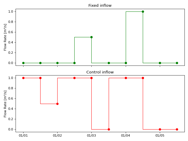
The desired outflow is set to be 1.0 cubic meter / second. The fixed inflow is ususally 0.0 except at a few moments. To get the desired output, the ideal controllable inflow is the outflow minus the fixed inflow shifted 24 hours in advance. The results are illustrated in the plot below.

(Source code, svg, png)

Note that the control inflow is 0.0 in the last 24 hours. The reason is that these values do not impact the outflow for the given time period anymore, due to the delay time of 24 hours.

For the simulation problem, we use the same model, but the control inflow is now given as input and is the same as the optimized inflow given by optimization problem. The simulation problem is given below.

class ExampleSim(CSVMixinSim, SimulationProblem):
    """
    A simulation problem example containing a delay component
    """

    timeseries_import_basename = "timeseries_import_simulation"
    timeseries_export_basename = "timeseries_export_simulation"

    def __init__(self, **kwargs):
        dt_hours = 12
        dt = dt_hours * 3600
        super().__init__(model_name="Example", fixed_dt=dt, **kwargs)

Note that for the simulation problem, we have to set the option fixed_dt. This is because currently optimization problems with delay equations only work for a fixed timestep size.

Since the model and inputs are the same, the volume output is exactly the same for both the simulation and optimization problem.