Mixed Integer Optimization: Pumps and Orifices
Note
This example focuses on how to incorporate mixed integer components into a hydraulic model, and assumes basic exposure to RTC-Tools. To start with basics, see Filling a Reservoir.
Note
By default, if you define any integer or boolean variables in the model, RTC-Tools
will switch from IPOPT to BONMIN. You can modify solver options by overriding
the
solver_options()
method. Refer to CasADi’s nlpsol interface for a list of supported solvers.
The Model
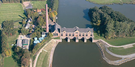
For this example, the model represents a typical setup for the dewatering of lowland areas. Water is routed from the hinterland (modeled as discharge boundary condition, right side) through a canal (modeled as storage element) towards the sea (modeled as water level boundary condition on the left side). Keeping the lowland area dry requires that enough water is discharged to the sea. If the sea water level is lower than the water level in the canal, the water can be discharged to the sea via gradient flow through the orifice (or a weir). If the sea water level is higher than in the canal, water must be pumped.
To discharge water via gradient flow is free, while pumping costs money. The control task is to keep the water level in the canal below a given flood warning level at minimum costs. The expected result is that the model computes a control pattern that makes use of gradient flow whenever possible and activates the pump only when necessary.
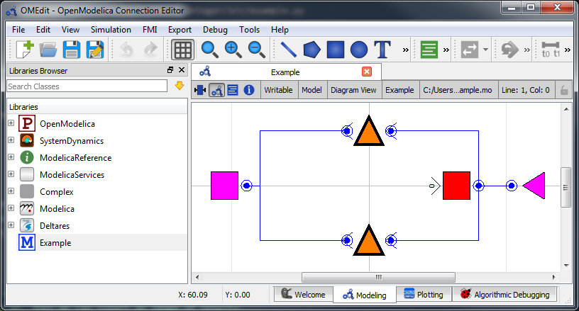
The model can be viewed and edited using the OpenModelica Connection Editor
program. First load the Deltares library into OpenModelica Connection Editor,
and then load the example model, located at
<examples directory>\mixed_integer\model\Example.mo. The model Example.mo
represents a simple water system with the following elements:
- a canal segment, modeled as storage element
Deltares.ChannelFlow.Hydraulic.Storage.Linear, - a discharge boundary condition
Deltares.ChannelFlow.Hydraulic.BoundaryConditions.Discharge, - a water level boundary condition
Deltares.ChannelFlow.Hydraulic.BoundaryConditions.Level, - a pump
Deltares.ChannelFlow.Hydraulic.Structures.Pump - an orifice modeled as a pump
Deltares.ChannelFlow.Hydraulic.Structures.Pump
In text mode, the Modelica model looks as follows (with annotation statements removed):
1 2 3 4 5 6 7 8 9 10 11 12 13 14 15 16 17 18 19 20 21 22 23 24 | model Example
// Declare Model Elements
Deltares.ChannelFlow.Hydraulic.Storage.Linear storage(A=1.0e6, H_b=0.0, HQ.H(min=0.0, max=0.5));
Deltares.ChannelFlow.Hydraulic.BoundaryConditions.Discharge discharge;
Deltares.ChannelFlow.Hydraulic.BoundaryConditions.Level level;
Deltares.ChannelFlow.Hydraulic.Structures.Pump pump;
Deltares.ChannelFlow.Hydraulic.Structures.Pump orifice;
// Define Input/Output Variables and set them equal to model variables
input Modelica.SIunits.VolumeFlowRate Q_pump(fixed=false, min=0.0, max=7.0) = pump.Q;
input Boolean is_downhill;
input Modelica.SIunits.VolumeFlowRate Q_in(fixed=true) = discharge.Q;
input Modelica.SIunits.Position H_sea(fixed=true) = level.H;
input Modelica.SIunits.VolumeFlowRate Q_orifice(fixed=false, min=0.0, max=10.0) = orifice.Q;
output Modelica.SIunits.Position storage_level = storage.HQ.H;
output Modelica.SIunits.Position sea_level = level.H;
equation
// Connect Model Elements
connect(orifice.HQDown, level.HQ);
connect(storage.HQ, orifice.HQUp);
connect(storage.HQ, pump.HQUp);
connect(discharge.HQ, storage.HQ);
connect(pump.HQDown, level.HQ);
end Example;
|
The five water system elements (storage, discharge boundary condition, water
level boundary condition, pump, and orifice) appear under the model Example
statement. The equation part connects these five elements with the help of
connections. Note that Pump extends the partial model HQTwoPort which
inherits from the connector HQPort. With HQTwoPort, Pump can be
connected on two sides. level represents a model boundary condition (model
is meant in a hydraulic sense here), so it can be connected to one other
element only. It extends the HQOnePort which again inherits from the
connector HQPort.
In addition to elements, the input variables Q_in, H_sea, Q_pump,
and Q_orifice are also defined. Because we want to view the water levels in
the storage element in the output file, we also define output
variables storage_level and sea_level. It is usually easiest to set input
and output variables equal to their corresponding model variable in the same line.
To maintain the linearity of the model, we input the Boolean is_downhill as
a way to keep track of whether water can flow by gravity to the sea. This
variable is not used directly in the hydraulics, but we use it later in the
constraints in the python file.
The Optimization Problem
The python script consists of the following blocks:
- Import of packages
- Definition of the optimization problem class
- Constructor
- Objective function
- Definition of constraints
- Additional configuration of the solver
- A run statement
Importing Packages
For this example, the import block is as follows:
1 2 3 4 5 6 | import numpy as np
from rtctools.optimization.collocated_integrated_optimization_problem \
import CollocatedIntegratedOptimizationProblem
from rtctools.optimization.csv_mixin import CSVMixin
from rtctools.optimization.modelica_mixin import ModelicaMixin
|
Note that we are also importing inf from numpy. We will use this later
in the constraints.
Optimization Problem
Next, we construct the class by declaring it and inheriting the desired parent classes.
10 | class Example(CSVMixin, ModelicaMixin, CollocatedIntegratedOptimizationProblem):
|
Now we define an objective function. This is a class method that returns the value that needs to be minimized. Here we specify that we want to minimize the volume pumped:
18 19 20 21 22 | def objective(self, ensemble_member):
# Minimize water pumped. The total water pumped is the integral of the
# water pumped from the starting time until the stoping time. In
# practice, self.integral() is a summation of all the discrete states.
return self.integral('Q_pump', ensemble_member)
|
Constraints can be declared by declaring the path_constraints() method.
Path constraints are constraints that are applied every timestep. To set a
constraint at an individual timestep, define it inside the constraints
method.
The orifice BooleanSubmergedOrifice requires special constraints to be set
in order to work. They are implemented below in the path_constraints()
method. their parent classes also declare this method, so we call the
super() method so that we don’t overwrite their behaviour.
26 27 28 29 30 31 32 33 34 35 36 37 38 39 40 41 42 43 44 45 46 47 48 49 50 51 52 53 54 55 56 57 58 | def path_constraints(self, ensemble_member):
# Call super to get default constraints
constraints = super().path_constraints(ensemble_member)
M = 2 # The so-called "big-M"
# Release through orifice downhill only. This constraint enforces the
# fact that water only flows downhill.
constraints.append(
(self.state('Q_orifice') + (1 - self.state('is_downhill')) * 10,
0.0, 10.0))
# Make sure is_downhill is true only when the sea is lower than the
# water level in the storage.
constraints.append((self.state('H_sea') - self.state('storage.HQ.H') -
(1 - self.state('is_downhill')) * M, -np.inf, 0.0))
constraints.append((self.state('H_sea') - self.state('storage.HQ.H') +
self.state('is_downhill') * M, 0.0, np.inf))
# Orifice flow constraint. Uses the equation:
# Q(HUp, HDown, d) = width * C * d * (2 * g * (HUp - HDown)) ^ 0.5
# Note that this equation is only valid for orifices that are submerged
# units: description:
w = 3.0 # m width of orifice
d = 0.8 # m hight of orifice
C = 1.0 # none orifice constant
g = 9.8 # m/s^2 gravitational acceleration
constraints.append(
(((self.state('Q_orifice') / (w * C * d)) ** 2) / (2 * g) +
self.state('orifice.HQDown.H') - self.state('orifice.HQUp.H') -
M * (1 - self.state('is_downhill')),
-np.inf, 0.0))
return constraints
|
Finally, we want to apply some additional configuration, reducing the amount of information the solver outputs:
61 62 63 64 65 66 | def solver_options(self):
options = super().solver_options()
# Restrict solver output
solver = options['solver']
options[solver]['print_level'] = 1
return options
|
Run the Optimization Problem
To make our script run, at the bottom of our file we just have to call
the run_optimization_problem() method we imported on the optimization
problem class we just created.
70 | run_optimization_problem(Example)
|
The Whole Script
All together, the whole example script is as follows:
1 2 3 4 5 6 7 8 9 10 11 12 13 14 15 16 17 18 19 20 21 22 23 24 25 26 27 28 29 30 31 32 33 34 35 36 37 38 39 40 41 42 43 44 45 46 47 48 49 50 51 52 53 54 55 56 57 58 59 60 61 62 63 64 65 66 67 68 69 70 | import numpy as np
from rtctools.optimization.collocated_integrated_optimization_problem \
import CollocatedIntegratedOptimizationProblem
from rtctools.optimization.csv_mixin import CSVMixin
from rtctools.optimization.modelica_mixin import ModelicaMixin
from rtctools.util import run_optimization_problem
class Example(CSVMixin, ModelicaMixin, CollocatedIntegratedOptimizationProblem):
"""
This class is the optimization problem for the Example. Within this class,
the objective, constraints and other options are defined.
"""
# This is a method that returns an expression for the objective function.
# RTC-Tools always minimizes the objective.
    def objective(self, ensemble_member):
        # Minimize water pumped. The total water pumped is the integral of the
        # water pumped from the starting time until the stoping time. In
        # practice, self.integral() is a summation of all the discrete states.
        return self.integral('Q_pump', ensemble_member)
# A path constraint is a constraint where the values in the constraint are a
# Timeseries rather than a single number.
    def path_constraints(self, ensemble_member):
        # Call super to get default constraints
        constraints = super().path_constraints(ensemble_member)
        M = 2  # The so-called "big-M"

        # Release through orifice downhill only. This constraint enforces the
        # fact that water only flows downhill.
        constraints.append(
            (self.state('Q_orifice') + (1 - self.state('is_downhill')) * 10,
             0.0, 10.0))

        # Make sure is_downhill is true only when the sea is lower than the
        # water level in the storage.
        constraints.append((self.state('H_sea') - self.state('storage.HQ.H') -
                            (1 - self.state('is_downhill')) * M, -np.inf, 0.0))
        constraints.append((self.state('H_sea') - self.state('storage.HQ.H') +
                            self.state('is_downhill') * M, 0.0, np.inf))

        # Orifice flow constraint. Uses the equation:
        # Q(HUp, HDown, d) = width * C * d * (2 * g * (HUp - HDown)) ^ 0.5
        # Note that this equation is only valid for orifices that are submerged
        #          units:  description:
        w = 3.0  # m       width of orifice
        d = 0.8  # m       hight of orifice
        C = 1.0  # none    orifice constant
        g = 9.8  # m/s^2   gravitational acceleration
        constraints.append(
            (((self.state('Q_orifice') / (w * C * d)) ** 2) / (2 * g) +
             self.state('orifice.HQDown.H') - self.state('orifice.HQUp.H') -
             M * (1 - self.state('is_downhill')),
             -np.inf, 0.0))

        return constraints
# Any solver options can be set here
    def solver_options(self):
        options = super().solver_options()
        # Restrict solver output
        solver = options['solver']
        options[solver]['print_level'] = 1
        return options
# Run
run_optimization_problem(Example)
|
Running the Optimization Problem
Note
An explaination of bonmin behaviour and output goes here.
Extracting Results
The results from the run are found in output/timeseries_export.csv. Any
CSV-reading software can import it, but this is how results can be plotted using
the python library matplotlib:
import numpy as np
import matplotlib.pyplot as plt
import matplotlib.dates as mdates
from datetime import datetime


data_path = '../../../examples/mixed_integer/output/timeseries_export.csv'
delimiter = ','

# Import Data
ncols = len(np.genfromtxt(data_path, max_rows=1, delimiter=delimiter))
datefunc = lambda x: datetime.strptime(x, '%Y-%m-%d %H:%M:%S')
results = np.genfromtxt(data_path, converters={0: datefunc}, delimiter=delimiter,
                        dtype='object' + ',float' * (ncols - 1), names=True, encoding=None)[1:]

# Generate Plot
f, axarr = plt.subplots(2, sharex=True)
axarr[0].set_title('Water Level and Discharge')

# Upper subplot
axarr[0].set_ylabel('Water Level [m]')
axarr[0].plot(results['time'], results['storage_level'], label='Storage',
              linewidth=2, color='b')
axarr[0].plot(results['time'], results['sea_level'], label='Sea',
              linewidth=2, color='m')
axarr[0].plot(results['time'], 0.5 * np.ones_like(results['time']), label='Storage Max',
              linewidth=2, color='r', linestyle='--')

# Lower Subplot
axarr[1].set_ylabel('Flow Rate [m³/s]')
axarr[1].plot(results['time'], results['Q_orifice'], label='Orifice',
              linewidth=2, color='g')
axarr[1].plot(results['time'], results['Q_pump'], label='Pump',
              linewidth=2, color='r')
axarr[1].xaxis.set_major_formatter(mdates.DateFormatter('%H:%M'))
f.autofmt_xdate()

# Shrink each axis by 20% and put a legend to the right of the axis
for i in range(len(axarr)):
    box = axarr[i].get_position()
    axarr[i].set_position([box.x0, box.y0, box.width * 0.8, box.height])
    axarr[i].legend(loc='center left', bbox_to_anchor=(1, 0.5), frameon=False)

plt.autoscale(enable=True, axis='x', tight=True)

# Output Plot
plt.show()
(Source code, png, hires.png, pdf)
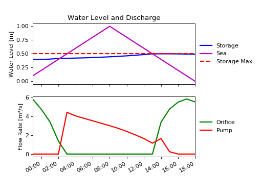
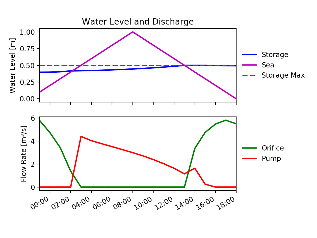
Observations
Note that in the results plotted above, the pump runs with a constantly varying throughput. To smooth out the flow through the pump, consider using goal programming to apply a path goal minimizing the derivative of the pump at each timestep. For an example, see the third goal in Declaring Goals.