Using an Ensemble Forecast
Note
This example is an extension of Using Lookup Tables. It assumes prior knowledge of goal programming and the lookup tables components of RTC-Tools. If you are a first-time user of RTC-Tools, see Filling a Reservoir.
Then biggest change to RTC-Tools when using an ensemble is the structure of the
directory. The folder <examples directory>\ensemble
contains a complete RTC-Tools ensemble optimization problem. An RTC-Tools
ensemble directory has the following structure:
model: This folder contains the Modelica model. The Modelica model contains the physics of the RTC-Tools model.src: This folder contains a Python file. This file contains the configuration of the model and is used to run the model.input: This folder contains the model input data pertaining to each ensemble member:ensemble.csv: a file where the names and probabilities of the ensemble members are definedforecast1- the file
timeseries_import.csv - the file
initial_state.csv
- the file
forecast2timeseries_import.csvinitial_state.csv
- …
output: The folder where the output is saved:forecast1timeseries_export.csv
forecast2timeseries_export.csv
- …
The Model
Note
This example uses the same hydraulic model as the basic example. For a detailed explanation of the hydraulic model, see Filling a Reservoir.
In OpenModelica Connection Editor, the model looks like this:
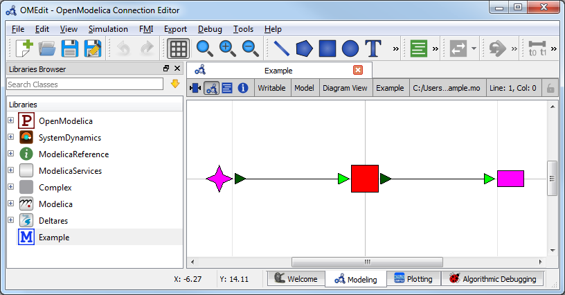
In text mode, the Modelica model is as follows (with annotation statements removed):
1 2 3 4 5 6 7 8 9 10 11 12 | model Example
Deltares.ChannelFlow.SimpleRouting.BoundaryConditions.Inflow inflow;
Deltares.ChannelFlow.SimpleRouting.Storage.Storage storage(V(nominal=4e5, min=2e5, max=6e5));
Deltares.ChannelFlow.SimpleRouting.BoundaryConditions.Terminal outfall;
input Modelica.SIunits.VolumeFlowRate Q_in(fixed = true);
input Modelica.SIunits.VolumeFlowRate Q_release(fixed = false, min = 0.0, max = 6.0);
equation
connect(inflow.QOut, storage.QIn);
connect(storage.QOut, outfall.QIn);
storage.Q_release = Q_release;
inflow.Q = Q_in;
end Example;
|
The Optimization Problem
The python script consists of the following blocks:
- Import of packages
- Declaration of Goals
- Declaration of the optimization problem class
- Constructor
- Set
csv_ensemble_mode = True - Declaration of a
pre()method - Specification of Goals
- Declaration of a
priority_completed()method - Declaration of a
post()method - Additional configuration of the solver
- A run statement
Importing Packages
For this example, the import block is as follows:
1 2 3 4 5 6 7 8 9 10 | import numpy as np
from rtctools.optimization.collocated_integrated_optimization_problem \
import CollocatedIntegratedOptimizationProblem
from rtctools.optimization.control_tree_mixin import ControlTreeMixin
from rtctools.optimization.csv_lookup_table_mixin import CSVLookupTableMixin
from rtctools.optimization.csv_mixin import CSVMixin
from rtctools.optimization.goal_programming_mixin \
import GoalProgrammingMixin, StateGoal
from rtctools.optimization.modelica_mixin import ModelicaMixin
|
Declaring Goals
First, we have a high priority goal to keep the water volume within a minimum and maximum.
14 15 16 17 18 19 20 21 | class WaterVolumeRangeGoal(StateGoal):
def __init__(self, optimization_problem):
# Assign V_min and V_max the the target range
self.target_min = optimization_problem.get_timeseries('V_min')
self.target_max = optimization_problem.get_timeseries('V_max')
super().__init__(optimization_problem)
state = 'storage.V'
priority = 1
|
We also want to save energy, so we define a goal to minimize Q_release. This
goal has a lower priority.
24 25 26 27 28 29 30 | class MinimizeQreleaseGoal(StateGoal):
# GoalProgrammingMixin will try to minimize the following state
state = 'Q_release'
# The lower the number returned by this function, the higher the priority.
priority = 2
# The penalty variable is taken to the order'th power.
order = 1
|
Optimization Problem
Next, we construct the class by declaring it and inheriting the desired parent classes.
33 34 | class Example(GoalProgrammingMixin, CSVMixin, CSVLookupTableMixin, ModelicaMixin,
ControlTreeMixin, CollocatedIntegratedOptimizationProblem):
|
We turn on ensemble mode by setting csv_ensemble_mode = True:
49 50 | ensemble_member: [] for ensemble_member in range(self.ensemble_size)}
|
The method pre() is already defined in RTC-Tools, but we would like to add
a line to it to create a variable for storing intermediate results. To do
this, we declare a new pre() method, call super().pre()
to ensure that the original method runs unmodified, and add in a variable
declaration to store our list of intermediate results. This variable is a
dict, reflecting the need to store results from multiple ensemble.
Because the timeseries we set will be the same for both ensemble members, we also make sure that the timeseries we set are set for both ensemble members using for loops.
42 43 44 45 46 47 48 49 50 51 52 53 54 55 56 57 58 59 60 61 62 63 64 65 66 67 68 69 70 71 72 73 74 | def pre(self):
# Do the standard preprocessing
super().pre()
# Create a dict of empty lists for storing intermediate results from
# each ensemble
self.intermediate_results = {
ensemble_member: [] for ensemble_member in range(self.ensemble_size)}
# Cache lookup tables for convenience and code legibility
_lookup_tables = self.lookup_tables(ensemble_member=0)
self.lookup_storage_V = _lookup_tables['storage_V']
# Non-varying goals can be implemented as a timeseries
for e_m in range(self.ensemble_size):
self.set_timeseries('H_min', np.ones_like(self.times()) * 0.44,
ensemble_member=e_m)
self.set_timeseries('H_max', np.ones_like(self.times()) * 0.46,
ensemble_member=e_m)
# Q_in is a varying input and is defined in each timeseries_import.csv
# However, if we set it again here, it will be added to the output files
self.set_timeseries('Q_in',
self.get_timeseries('Q_in', ensemble_member=e_m),
ensemble_member=e_m)
# Convert our water level goals into volume goals
self.set_timeseries('V_max',
self.lookup_storage_V(self.get_timeseries('H_max')),
ensemble_member=e_m)
self.set_timeseries('V_min',
self.lookup_storage_V(self.get_timeseries('H_min')),
ensemble_member=e_m)
|
Now we pass in the goals:
76 77 78 79 80 | def path_goals(self):
g = []
g.append(WaterVolumeRangeGoal(self))
g.append(MinimizeQreleaseGoal(self))
return g
|
In order to better demonstrate the way that ensembles are handled in RTC-
Tools, we modify the control_tree_options() method. The default setting
allows the control tree to split at every time, but we override this method
and force it to split at a single timestep. See Observations at
the bottom of the page for more information.
82 83 84 85 86 87 88 | def control_tree_options(self):
# We want to modify the control tree options, so we override the default
# control_tree_options method. We call super() to get the default options
options = super().control_tree_options()
# Change the branching_times list to only contain the fifth timestep
options['branching_times'] = [self.times()[5]]
return options
|
We define the priority_completed() method. We ensure that it stores the
results from both ensemble members.
90 91 92 93 94 95 96 97 98 99 100 101 102 103 104 105 106 107 108 109 110 111 | def priority_completed(self, priority):
# We want to print some information about our goal programming problem.
# We store the useful numbers temporarily, and print information at the
# end of our run.
for e_m in range(self.ensemble_size):
results = self.extract_results(e_m)
self.set_timeseries('V_storage', results['storage.V'], ensemble_member=e_m)
_max = self.get_timeseries('V_max', ensemble_member=e_m).values
_min = self.get_timeseries('V_min', ensemble_member=e_m).values
V_storage = self.get_timeseries('V_storage', ensemble_member=e_m).values
# A little bit of tolerance when checking for acceptance. This
# tolerance must be set greater than the tolerance of the solver.
tol = 10
_max += tol
_min -= tol
n_level_satisfied = sum(
np.logical_and(_min <= V_storage, V_storage <= _max))
q_release_integral = sum(results['Q_release'])
self.intermediate_results[e_m].append((priority, n_level_satisfied,
q_release_integral))
|
We output our intermediate results using the post() method:
113 114 115 116 117 118 119 120 121 122 | def post(self):
super().post()
for e_m in range(self.ensemble_size):
print('\n\nResults for Ensemble Member {}:'.format(e_m))
for priority, n_level_satisfied, q_release_integral in \
self.intermediate_results[e_m]:
print("\nAfter finishing goals of priority {}:".format(priority))
print("Level goal satisfied at {} of {} time steps".format(
n_level_satisfied, len(self.times())))
print("Integral of Q_release = {:.2f}".format(q_release_integral))
|
Finally, we want to apply some additional configuration, reducing the amount of information the solver outputs:
125 126 127 128 129 130 131 132 133 | def solver_options(self):
options = super().solver_options()
# When mumps_scaling is not zero, errors occur. RTC-Tools does its own
# scaling, so mumps scaling is not critical. Proprietary HSL solvers
# do not exhibit this error.
solver = options['solver']
options[solver]['mumps_scaling'] = 0
options[solver]['print_level'] = 1
return options
|
Run the Optimization Problem
To make our script run, at the bottom of our file we just have to call
the run_optimization_problem() method we imported on the optimization
problem class we just created.
137 | run_optimization_problem(Example)
|
The Whole Script
All together, the whole example script is as follows:
1 2 3 4 5 6 7 8 9 10 11 12 13 14 15 16 17 18 19 20 21 22 23 24 25 26 27 28 29 30 31 32 33 34 35 36 37 38 39 40 41 42 43 44 45 46 47 48 49 50 51 52 53 54 55 56 57 58 59 60 61 62 63 64 65 66 67 68 69 70 71 72 73 74 75 76 77 78 79 80 81 82 83 84 85 86 87 88 89 90 91 92 93 94 95 96 97 98 99 100 101 102 103 104 105 106 107 108 109 110 111 112 113 114 115 116 117 118 119 120 121 122 123 124 125 126 127 128 129 130 131 132 133 134 135 136 137 | import numpy as np
from rtctools.optimization.collocated_integrated_optimization_problem \
import CollocatedIntegratedOptimizationProblem
from rtctools.optimization.control_tree_mixin import ControlTreeMixin
from rtctools.optimization.csv_lookup_table_mixin import CSVLookupTableMixin
from rtctools.optimization.csv_mixin import CSVMixin
from rtctools.optimization.goal_programming_mixin \
import GoalProgrammingMixin, StateGoal
from rtctools.optimization.modelica_mixin import ModelicaMixin
from rtctools.util import run_optimization_problem
class WaterVolumeRangeGoal(StateGoal):
    def __init__(self, optimization_problem):
        # Assign V_min and V_max the the target range
        self.target_min = optimization_problem.get_timeseries('V_min')
        self.target_max = optimization_problem.get_timeseries('V_max')
        super().__init__(optimization_problem)
    state = 'storage.V'
    priority = 1
class MinimizeQreleaseGoal(StateGoal):
    # GoalProgrammingMixin will try to minimize the following state
    state = 'Q_release'
    # The lower the number returned by this function, the higher the priority.
    priority = 2
    # The penalty variable is taken to the order'th power.
    order = 1
class Example(GoalProgrammingMixin, CSVMixin, CSVLookupTableMixin, ModelicaMixin,
              ControlTreeMixin, CollocatedIntegratedOptimizationProblem):
"""
An extention of the goal programming and lookuptable examples that
demonstrates how to work with ensembles.
"""
# Overide default csv_ensemble_mode = False from CSVMixin before calling pre()
csv_ensemble_mode = True
    def pre(self):
        # Do the standard preprocessing
        super().pre()

        # Create a dict of empty lists for storing intermediate results from
        # each ensemble
        self.intermediate_results = {
            ensemble_member: [] for ensemble_member in range(self.ensemble_size)}

        # Cache lookup tables for convenience and code legibility
        _lookup_tables = self.lookup_tables(ensemble_member=0)
        self.lookup_storage_V = _lookup_tables['storage_V']

        # Non-varying goals can be implemented as a timeseries
        for e_m in range(self.ensemble_size):
            self.set_timeseries('H_min', np.ones_like(self.times()) * 0.44,
                                ensemble_member=e_m)
            self.set_timeseries('H_max', np.ones_like(self.times()) * 0.46,
                                ensemble_member=e_m)

            # Q_in is a varying input and is defined in each timeseries_import.csv
            # However, if we set it again here, it will be added to the output files
            self.set_timeseries('Q_in',
                                self.get_timeseries('Q_in', ensemble_member=e_m),
                                ensemble_member=e_m)

            # Convert our water level goals into volume goals
            self.set_timeseries('V_max',
                                self.lookup_storage_V(self.get_timeseries('H_max')),
                                ensemble_member=e_m)
            self.set_timeseries('V_min',
                                self.lookup_storage_V(self.get_timeseries('H_min')),
                                ensemble_member=e_m)
    def path_goals(self):
        g = []
        g.append(WaterVolumeRangeGoal(self))
        g.append(MinimizeQreleaseGoal(self))
        return g
    def control_tree_options(self):
        # We want to modify the control tree options, so we override the default
        # control_tree_options method. We call super() to get the default options
        options = super().control_tree_options()
        # Change the branching_times list to only contain the fifth timestep
        options['branching_times'] = [self.times()[5]]
        return options
    def priority_completed(self, priority):
        # We want to print some information about our goal programming problem.
        # We store the useful numbers temporarily, and print information at the
        # end of our run.
        for e_m in range(self.ensemble_size):
            results = self.extract_results(e_m)
            self.set_timeseries('V_storage', results['storage.V'], ensemble_member=e_m)

            _max = self.get_timeseries('V_max', ensemble_member=e_m).values
            _min = self.get_timeseries('V_min', ensemble_member=e_m).values
            V_storage = self.get_timeseries('V_storage', ensemble_member=e_m).values

            # A little bit of tolerance when checking for acceptance. This
            # tolerance must be set greater than the tolerance of the solver.
            tol = 10
            _max += tol
            _min -= tol
            n_level_satisfied = sum(
                np.logical_and(_min <= V_storage, V_storage <= _max))
            q_release_integral = sum(results['Q_release'])
            self.intermediate_results[e_m].append((priority, n_level_satisfied,
                                                   q_release_integral))
    def post(self):
        super().post()
        for e_m in range(self.ensemble_size):
            print('\n\nResults for Ensemble Member {}:'.format(e_m))
            for priority, n_level_satisfied, q_release_integral in \
                    self.intermediate_results[e_m]:
                print("\nAfter finishing goals of priority {}:".format(priority))
                print("Level goal satisfied at {} of {} time steps".format(
                    n_level_satisfied, len(self.times())))
                print("Integral of Q_release = {:.2f}".format(q_release_integral))
# Any solver options can be set here
    def solver_options(self):
        options = super().solver_options()
        # When mumps_scaling is not zero, errors occur. RTC-Tools does its own
        # scaling, so mumps scaling is not critical. Proprietary HSL solvers
        # do not exhibit this error.
        solver = options['solver']
        options[solver]['mumps_scaling'] = 0
        options[solver]['print_level'] = 1
        return options
# Run
run_optimization_problem(Example)
|
Running the Optimization Problem
Following the execution of the optimization problem, the post() method
should print out the following lines:
Results for Ensemble Member 0:

After finishing goals of priority 1:
Level goal satisfied at 10 of 12 time steps
Integral of Q_release = 17.34

After finishing goals of priority 2:
Level goal satisfied at 9 of 12 time steps
Integral of Q_release = 17.12


Results for Ensemble Member 1:

After finishing goals of priority 1:
Level goal satisfied at 10 of 12 time steps
Integral of Q_release = 20.82

After finishing goals of priority 2:
Level goal satisfied at 9 of 12 time steps
Integral of Q_release = 20.60
This is the same output as the output for Mixed Integer Optimization: Pumps and Orifices, except now the output for each ensemble is printed.
Extracting Results
The results from the run are found in output/forecast1/timeseries_export.csv
and output/forecast2/timeseries_export.csv. Any CSV-reading software can
import it, but this is how results can be plotted using the python library
matplotlib:
import numpy as np
import matplotlib.pyplot as plt
import matplotlib.dates as mdates
from datetime import datetime
from pylab import get_cmap

forecast_names = ['forecast1', 'forecast2']

# Import Data
def get_results(forecast_name):
    output_dir = '../../../examples/ensemble/output/'
    data_path = output_dir + forecast_name + '/timeseries_export.csv'
    delimiter = ','
    ncols = len(np.genfromtxt(data_path, max_rows=1, delimiter=delimiter))
    datefunc = lambda x: datetime.strptime(x, '%Y-%m-%d %H:%M:%S')
    return np.genfromtxt(data_path, converters={0: datefunc}, delimiter=delimiter,
                            dtype='object' + ',float' * (ncols - 1), names=True, encoding=None)

# Generate Plot
n_subplots = 2
f, axarr = plt.subplots(n_subplots, sharex=True, figsize=(8, 4 * n_subplots))
axarr[0].set_title('Water Volume and Discharge')
cmaps = ['Blues', 'Greens']
shades = [0.5, 0.8]
f.autofmt_xdate()

# Upper Subplot
axarr[0].set_ylabel('Water Volume in Storage [m³]')
axarr[0].ticklabel_format(style='sci', axis='y', scilimits=(0, 0))

# Lower Subplot
axarr[1].set_ylabel('Flow Rate [m³/s]')

# Plot Ensemble Members
for idx, forecast in enumerate(forecast_names):
    # Upper Subplot
    results = get_results(forecast)
    if idx == 0:
        axarr[0].plot(results['time'], results['V_max'], label='Max',
        linewidth=2, color='r', linestyle='--')
        axarr[0].plot(results['time'], results['V_min'], label='Min',
        linewidth=2, color='g', linestyle='--')
    axarr[0].plot(results['time'], results['V_storage'], label=forecast + ':Volume',
                        linewidth=2, color=get_cmap(cmaps[idx])(shades[1]))
    # Lower Subplot
    axarr[1].plot(results['time'], results['Q_in'], label='{}:Inflow'.format(forecast),
                            linewidth=2, color=get_cmap(cmaps[idx])(shades[0]))
    axarr[1].plot(results['time'], results['Q_release'], label='{}:Release'.format(forecast),
                            linewidth=2, color=get_cmap(cmaps[idx])(shades[1]))

# Shrink each axis by 30% and put a legend to the right of the axis
for i in range(len(axarr)):
    box = axarr[i].get_position()
    axarr[i].set_position([box.x0, box.y0, box.width * 0.7, box.height])
    axarr[i].legend(loc='center left', bbox_to_anchor=(1, 0.5), frameon=False)

plt.autoscale(enable=True, axis='x', tight=True)

# Output Plot
plt.show()
(Source code, png, hires.png, pdf)

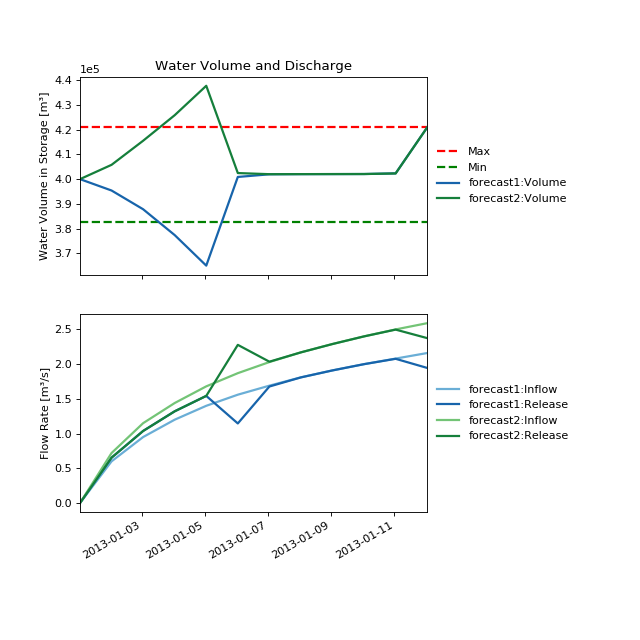
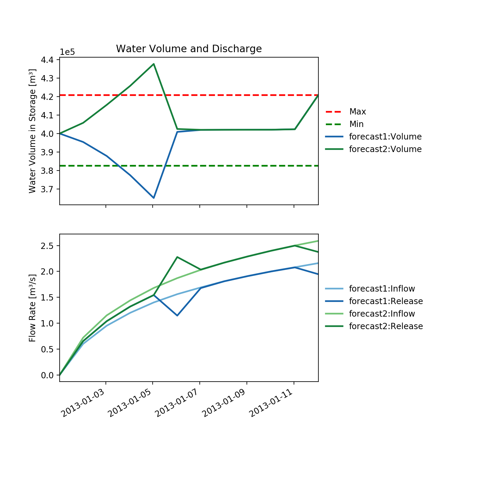
Observations
Note that in the results plotted above, the control tree follows a single path and does not branch until it arrives at the first branching time. Up until the branching point, RTC-Tools is making decisions that enhance the flexibility of the system so that it can respond as ideally as possible to whichever future emerges. In the case of two forecasts, this means taking a path that falls between the two possible futures. This will cause the water level to diverge from the ideal levels as time progresses. While this appears to be suboptimal, it is preferable to simply gambling on one of the forecasts coming true and ignoring the other. Once the branching time is reached, RTC-Tools is allowed to optimize for each individual branch separately. Immediately, RTC-Tools applies the corrective control needed to get the water levels into the acceptable range. If the operator simply picks a forecast to use and guesses wrong, the corrective control will have to be much more drastic and potentially catastrophic.