Using Lookup Tables
Note
This example focuses on how to implement non-linear storage elements in RTC-Tools using lookup tables. It assumes basic exposure to RTC-Tools. If you are a first-time user of RTC-Tools, see Filling a Reservoir.
This example also uses goal programming in the formulation. If you are unfamiliar with goal programming, please see Goal Programming: Defining Multiple Objectives.
The Model
Note
This example uses the same hydraulic model as the basic example. For a detalied explaination of the hydraulic model, see Filling a Reservoir.
In OpenModelica Connection Editor, the model looks like this:
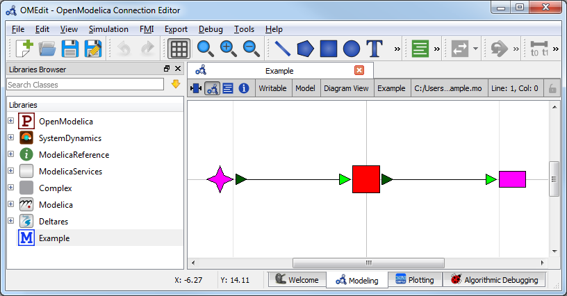
In text mode, the Modelica model is as follows (with annotation statements removed):
1 2 3 4 5 6 7 8 9 10 11 12 | model Example
Deltares.ChannelFlow.SimpleRouting.BoundaryConditions.Inflow inflow;
Deltares.ChannelFlow.SimpleRouting.Storage.Storage storage(V(nominal=4e5, min=2e5, max=6e5));
Deltares.ChannelFlow.SimpleRouting.BoundaryConditions.Terminal outfall;
input Modelica.SIunits.VolumeFlowRate Q_in(fixed = true);
input Modelica.SIunits.VolumeFlowRate Q_release(fixed = false, min = 0.0, max = 10.0);
equation
connect(inflow.QOut, storage.QIn);
connect(storage.QOut, outfall.QIn);
storage.Q_release = Q_release;
inflow.Q = Q_in;
end Example;
|
The Optimization Problem
The python script consists of the following blocks:
- Import of packages
- Declaration of Goals
- Declaration of the optimization problem class
- Constructor
- Declaration of a
pre()method - Specification of Goals
- Declaration of a
priority_completed()method - Declaration of a
post()method - Additional configuration of the solver
- A run statement
Importing Packages
For this example, the import block is as follows:
1 2 3 4 5 6 7 8 9 | import numpy as np
from rtctools.optimization.collocated_integrated_optimization_problem \
import CollocatedIntegratedOptimizationProblem
from rtctools.optimization.csv_lookup_table_mixin import CSVLookupTableMixin
from rtctools.optimization.csv_mixin import CSVMixin
from rtctools.optimization.goal_programming_mixin \
import GoalProgrammingMixin, StateGoal
from rtctools.optimization.modelica_mixin import ModelicaMixin
|
Declaring Goals
Goals are defined as classes that inherit the Goal parent class. The
components of goals can be found in Multi-objective optimization. In
this example, we use the helper goal class, StateGoal.
First, we have a high priority goal to keep the water volume within a minimum and maximum. We use a water volume goal instead of a water level goal when the volume-storage relation of the storage element is non-linear. The volume of water in the storage element behaves linearly, while the water level does not.
However, goals are usually defined in the form of water level goals. We will
convert the water level goals into volume goals within the optimization
problem class, so we define the __init__() method so we can pass the
values of the goals in later. We call the super() method to avoid
overwriting the __init__() method of the parent class.
13 14 15 16 17 18 19 20 21 22 23 24 25 | class WaterVolumeRangeGoal(StateGoal):
# We want to add a water volume range goal to our optimization. However, at
# the time of defining this goal we still do not know what the value of the
# min and max are. We add an __init__() method so that the values of these
# goals can be defined when the optimization problem class instantiates
# this goal.
def __init__(self, optimization_problem):
# Assign V_min and V_max the the target range
self.target_min = optimization_problem.get_timeseries('V_min')
self.target_max = optimization_problem.get_timeseries('V_max')
super().__init__(optimization_problem)
state = 'storage.V'
priority = 1
|
We also want to save energy, so we define a goal to minimize Q_release. This
goal has a lower priority.
28 29 30 31 32 33 34 | class MinimizeQreleaseGoal(StateGoal):
# GoalProgrammingMixin will try to minimize the following state:
state = 'Q_release'
# The lower the number returned by this function, the higher the priority.
priority = 2
# The penalty variable is taken to the order'th power.
order = 1
|
Optimization Problem
Next, we construct the class by declaring it and inheriting the desired parent classes.
37 38 | class Example(GoalProgrammingMixin, CSVLookupTableMixin, CSVMixin,
ModelicaMixin, CollocatedIntegratedOptimizationProblem):
|
The method pre() is already defined in RTC-Tools, but we would like to add
a line to it to create a variable for storing intermediate results. To do this,
we declare a new pre() method, call super().pre() to ensure
that the original method runs unmodified, and add in a variable declaration to
store our list of intermediate results.
We also want to convert our water level rane goal into a water volume range
goal. We can access the spline function describing the water level-storage
relation using the lookup_table() method. We cache the functions for
convenience. The lookup_storage_V() method can convert timeseries objects,
and we save the water volume goal bounds as timeseries.
44 45 46 47 48 49 50 51 52 53 54 55 56 57 58 59 60 61 62 63 64 | def pre(self):
super().pre()
# Empty list for storing intermediate_results
self.intermediate_results = []
# Cache lookup tables for convenience and legibility
_lookup_tables = self.lookup_tables(ensemble_member=0)
self.lookup_storage_V = _lookup_tables['storage_V']
# Non-varrying goals can be implemented as a timeseries like this:
self.set_timeseries('H_min', np.ones_like(self.times()) * 0.44, output=False)
# Q_in is a varying input and is defined in timeseries_import.csv
# However, if we set it again here, it will be added to the output file
self.set_timeseries('Q_in', self.get_timeseries('Q_in'))
# Convert our water level constraints into volume constraints
self.set_timeseries('V_max',
self.lookup_storage_V(self.get_timeseries('H_max')))
self.set_timeseries('V_min',
self.lookup_storage_V(self.get_timeseries('H_min')))
|
Notice that H_max was not defined in pre(). This is because it was defined as a timeseries import. We access timeseries using get_timeseries() and store them using set_timeseries(). Once a timeseries is set, we can access it later. In addition, all timeseries that are set are automatically included in the output file. You can find more information on timeseries here Basics.
Now we pass in the goals. We want to apply our goals to every timestep, so we
use the path_goals() method. This is a method that returns a list of the
goals we defined above. The WaterVolumeRangeGoal needs to be instantiated
with the new water volume timeseries we just defined.
66 67 68 69 70 | def path_goals(self):
g = []
g.append(WaterVolumeRangeGoal(self))
g.append(MinimizeQreleaseGoal(self))
return g
|
If all we cared about were the results, we could end our class declaration here. However, it is usually helpful to track how the solution changes after optimizing each priority level. To track these changes, we need to add three methods.
We define the priority_completed() method to inspect and summerize the
results. These are appended to our intermediate results variable after each
priority is completed.
75 76 77 78 79 80 81 82 83 84 85 86 87 88 89 90 91 | def priority_completed(self, priority):
results = self.extract_results()
self.set_timeseries('storage_V', results['storage.V'])
_max = self.get_timeseries('V_max').values
_min = self.get_timeseries('V_min').values
storage_V = self.get_timeseries('storage_V').values
# A little bit of tolerance when checking for acceptance.
tol = 10
_max += tol
_min -= tol
n_level_satisfied = sum(
np.logical_and(_min <= storage_V, storage_V <= _max))
q_release_integral = sum(results['Q_release'])
self.intermediate_results.append(
(priority, n_level_satisfied, q_release_integral))
|
We output our intermediate results using the post() method. Again, we nedd
to call the super() method to avoid overwiting the internal method.
93 94 95 96 97 98 99 100 | def post(self):
# Call super() class to not overwrite default behaviour
super().post()
for priority, n_level_satisfied, q_release_integral in self.intermediate_results:
print("\nAfter finishing goals of priority {}:".format(priority))
print("Volume goal satisfied at {} of {} time steps".format(
n_level_satisfied, len(self.times())))
print("Integral of Q_release = {:.2f}".format(q_release_integral))
|
Finally, we want to apply some additional configuration, reducing the amount of information the solver outputs:
103 104 105 106 107 | def solver_options(self):
options = super().solver_options()
solver = options['solver']
options[solver]['print_level'] = 1
return options
|
Run the Optimization Problem
To make our script run, at the bottom of our file we just have to call
the run_optimization_problem() method we imported on the optimization
problem class we just created.
111 | run_optimization_problem(Example)
|
The Whole Script
All together, the whole example script is as follows:
1 2 3 4 5 6 7 8 9 10 11 12 13 14 15 16 17 18 19 20 21 22 23 24 25 26 27 28 29 30 31 32 33 34 35 36 37 38 39 40 41 42 43 44 45 46 47 48 49 50 51 52 53 54 55 56 57 58 59 60 61 62 63 64 65 66 67 68 69 70 71 72 73 74 75 76 77 78 79 80 81 82 83 84 85 86 87 88 89 90 91 92 93 94 95 96 97 98 99 100 101 102 103 104 105 106 107 108 109 110 111 | import numpy as np
from rtctools.optimization.collocated_integrated_optimization_problem \
import CollocatedIntegratedOptimizationProblem
from rtctools.optimization.csv_lookup_table_mixin import CSVLookupTableMixin
from rtctools.optimization.csv_mixin import CSVMixin
from rtctools.optimization.goal_programming_mixin \
import GoalProgrammingMixin, StateGoal
from rtctools.optimization.modelica_mixin import ModelicaMixin
from rtctools.util import run_optimization_problem
class WaterVolumeRangeGoal(StateGoal):
    # We want to add a water volume range goal to our optimization. However, at
    # the time of defining this goal we still do not know what the value of the
    # min and max are. We add an __init__() method so that the values of these
    # goals can be defined when the optimization problem class instantiates
    # this goal.
    def __init__(self, optimization_problem):
        # Assign V_min and V_max the the target range
        self.target_min = optimization_problem.get_timeseries('V_min')
        self.target_max = optimization_problem.get_timeseries('V_max')
        super().__init__(optimization_problem)
    state = 'storage.V'
    priority = 1
class MinimizeQreleaseGoal(StateGoal):
    # GoalProgrammingMixin will try to minimize the following state:
    state = 'Q_release'
    # The lower the number returned by this function, the higher the priority.
    priority = 2
    # The penalty variable is taken to the order'th power.
    order = 1
class Example(GoalProgrammingMixin, CSVLookupTableMixin, CSVMixin,
              ModelicaMixin, CollocatedIntegratedOptimizationProblem):
"""
An extention of the goal programming example that shows how to incorporate
non-linear storage elements in the model.
"""
    def pre(self):
        super().pre()
        # Empty list for storing intermediate_results
        self.intermediate_results = []

        # Cache lookup tables for convenience and legibility
        _lookup_tables = self.lookup_tables(ensemble_member=0)
        self.lookup_storage_V = _lookup_tables['storage_V']

        # Non-varrying goals can be implemented as a timeseries like this:
        self.set_timeseries('H_min', np.ones_like(self.times()) * 0.44, output=False)

        # Q_in is a varying input and is defined in timeseries_import.csv
        # However, if we set it again here, it will be added to the output file
        self.set_timeseries('Q_in', self.get_timeseries('Q_in'))

        # Convert our water level constraints into volume constraints
        self.set_timeseries('V_max',
                            self.lookup_storage_V(self.get_timeseries('H_max')))
        self.set_timeseries('V_min',
                            self.lookup_storage_V(self.get_timeseries('H_min')))
    def path_goals(self):
        g = []
        g.append(WaterVolumeRangeGoal(self))
        g.append(MinimizeQreleaseGoal(self))
        return g
# We want to print some information about our goal programming problem. We
# store the useful numbers temporarily, and print information at the end of
# our run (see post() method below).
    def priority_completed(self, priority):
        results = self.extract_results()
        self.set_timeseries('storage_V', results['storage.V'])

        _max = self.get_timeseries('V_max').values
        _min = self.get_timeseries('V_min').values
        storage_V = self.get_timeseries('storage_V').values

        # A little bit of tolerance when checking for acceptance.
        tol = 10
        _max += tol
        _min -= tol
        n_level_satisfied = sum(
            np.logical_and(_min <= storage_V, storage_V <= _max))
        q_release_integral = sum(results['Q_release'])
        self.intermediate_results.append(
            (priority, n_level_satisfied, q_release_integral))
    def post(self):
        # Call super() class to not overwrite default behaviour
        super().post()
        for priority, n_level_satisfied, q_release_integral in self.intermediate_results:
            print("\nAfter finishing goals of priority {}:".format(priority))
            print("Volume goal satisfied at {} of {} time steps".format(
                n_level_satisfied, len(self.times())))
            print("Integral of Q_release = {:.2f}".format(q_release_integral))
# Any solver options can be set here
    def solver_options(self):
        options = super().solver_options()
        solver = options['solver']
        options[solver]['print_level'] = 1
        return options
# Run
run_optimization_problem(Example)
|
Running the Optimization Problem
Following the execution of the optimization problem, the post() method
should print out the following lines:
After finishing goals of priority 1:
Volume goal satisfied at 12 of 12 time steps
Integral of Q_release = 42.69

After finishing goals of priority 2:
Volume goal satisfied at 12 of 12 time steps
Integral of Q_release = 42.58
As the output indicates, while optimizing for the priority 1 goal, no attempt
was made to minimize the integral of Q_release. The only objective was to
minimize the number of states in violation of the water level goal.
After optimizing for the priority 2 goal, the solver was able to find a solution
that reduced the integral of Q_release without increasing the number of
timesteps where the water level exceded the limit.
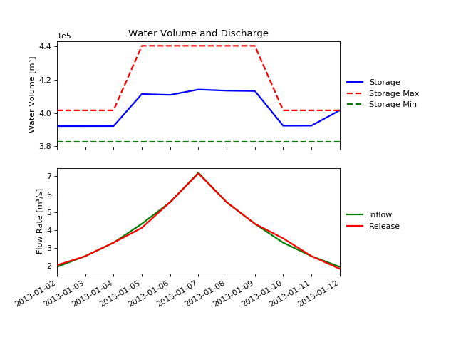
Extracting Results
The results from the run are found in output/timeseries_export.csv. Any
CSV-reading software can import it, but this is how results can be plotted using
the python library matplotlib:
import numpy as np
import matplotlib.pyplot as plt
import matplotlib.dates as mdates
from datetime import datetime


data_path = '../../../examples/lookup_table/output/timeseries_export.csv'
delimiter = ','

# Import Data
ncols = len(np.genfromtxt(data_path, max_rows=1, delimiter=delimiter))
datefunc = lambda x: datetime.strptime(x, '%Y-%m-%d %H:%M:%S')
results = np.genfromtxt(data_path, converters={0: datefunc}, delimiter=delimiter,
                        dtype='object' + ',float' * (ncols - 1), names=True, encoding=None)[1:]

# Generate Plot
n_subplots = 2
f, axarr = plt.subplots(n_subplots, sharex=True, figsize=(8, 3 * n_subplots))
axarr[0].set_title('Water Volume and Discharge')
f.autofmt_xdate()

# Upper subplot
axarr[0].set_ylabel('Water Volume [m³]')
axarr[0].ticklabel_format(style='sci', axis='y', scilimits=(0, 0))
axarr[0].plot(results['time'], results['storage_V'], label='Storage',
              linewidth=2, color='b')
axarr[0].plot(results['time'], results['V_max'], label='Storage Max',
              linewidth=2, color='r', linestyle='--')
axarr[0].plot(results['time'], results['V_min'], label='Storage Min',
              linewidth=2, color='g', linestyle='--')

# Lower Subplot
axarr[1].set_ylabel('Flow Rate [m³/s]')
axarr[1].plot(results['time'], results['Q_in'], label='Inflow',
              linewidth=2, color='g')
axarr[1].plot(results['time'], results['Q_release'], label='Release',
              linewidth=2, color='r')

# Shrink each axis by 20% and put a legend to the right of the axis
for i in range(n_subplots):
    box = axarr[i].get_position()
    axarr[i].set_position([box.x0, box.y0, box.width * 0.8, box.height])
    axarr[i].legend(loc='center left', bbox_to_anchor=(1, 0.5), frameon=False)

plt.autoscale(enable=True, axis='x', tight=True)

# Output Plot
plt.show()
(Source code, png, hires.png, pdf)