Tracking a Setpoint
Overview
The purpose of this example is to understand the technical setup of an RTC- Tools simulation model, how to run the model, and how to access the results.
The scenario is the following: A reservoir operator is trying to keep the reservoir’s volume close to a given target volume. They are given a six-day forecast of inflows given in 12-hour increments. To keep things simple, we ignore the waterlevel-storage relation of the reservoir and head-discharge relationships in this example. To make things interesting, the reservoir operator is only able to release water at a few discrete flow rates, and only change the discrete flow rate every 12 hours. They have chosen to use the RTC- Tools simulator to see if a simple proportional controller will be able to keep the system close enough to the target water volume.
The folder <examples directory>\simulation
contains a complete RTC-Tools simulation problem. An RTC-Tools
directory has the following structure:
input: This folder contains the model input data. These are several files in comma separated value format,csv.model: This folder contains the Modelica model. The Modelica model contains the physics of the RTC-Tools model.output: The folder where the output is saved in the filetimeseries_export.csv.src: This folder contains a Python file. This file contains the configuration of the model and is used to run the model .
The Model
The first step is to develop a physical model of the system. The model can be viewed and edited using the OpenModelica Connection Editor (OMEdit) program. For how to download and start up OMEdit, see Getting OMEdit.
Make sure to load the Deltares library before loading the example:
Load the Deltares library into OMEdit
Using the menu bar: File -> Open Model/Library File(s)
Select
<library directory>\Deltares\package.mo
Load the example model into OMEdit
Using the menu bar: File -> Open Model/Library File(s)
Select
<examples directory\simulation\model\Example.mo
Once loaded, we have an OpenModelica Connection Editor window that looks like this:
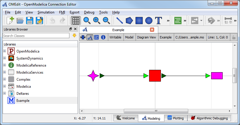
The model Example.mo represents a simple system with the following
elements:
a reservoir, modeled as storage element
Deltares.ChannelFlow.SimpleRouting.Storage.Storage,an inflow boundary condition
Deltares.ChannelFlow.SimpleRouting.BoundaryConditions.Inflow,an outfall boundary condition
Deltares.ChannelFlow.SimpleRouting.BoundaryConditions.Terminal,connectors (black lines) connecting the elements.
You can use the mouse-over feature help to identify the predefined models from the Deltares library. You can also drag the elements around- the connectors will move with the elements. Adding new elements is easy- just drag them in from the Deltares Library on the sidebar. Connecting the elements is just as easy- click and drag between the ports on the elements.
In text mode, the Modelica model looks as follows (with annotation statements removed):
 1model Example
 2  // Elements
 3  Deltares.ChannelFlow.SimpleRouting.BoundaryConditions.Inflow inflow(Q = Q_in);
 4  Deltares.ChannelFlow.SimpleRouting.Storage.Storage storage(Q_release = P_control, V(start=storage_V_init, fixed=true, nominal=4e5));
 5  Deltares.ChannelFlow.SimpleRouting.BoundaryConditions.Terminal outfall;
 6  // Initial States
 7  parameter Modelica.Units.SI.Volume storage_V_init;
 8  // Inputs
 9  input Modelica.Units.SI.VolumeFlowRate P_control(fixed = true);
10  input Modelica.Units.SI.VolumeFlowRate Q_in(fixed = true);
11  input Modelica.Units.SI.VolumeFlowRate storage_V_target(fixed = true);
12  // Outputs
13  output Modelica.Units.SI.Volume storage_V = storage.V;
14  output Modelica.Units.SI.VolumeFlowRate Q_release = P_control;
15equation
16  connect(inflow.QOut, storage.QIn);
17  connect(storage.QOut, outfall.QIn);
18end Example;
The three water system elements (storage, inflow, and outfall) appear under
the model Example statement. The equation part connects these three
elements with the help of connections. Note that storage extends the partial
model QSISO which contains the connectors QIn and QOut.
With QSISO, storage can be connected on two sides. The storage
element also has a variable Q_release, which is the decision variable the
operator controls.
OpenModelica Connection Editor will automatically generate the element and
connector entries in the text text file. Defining inputs and outputs requires
editing the text file directly and assigning the inputs to the appropriate
element variables. For example, inflow(Q = Q_in) sets the Q variable
of the inflow element equal to Q_in.
In addition to elements, the input variables Q_in and P_control are
also defined. Q_in is determined by the forecast and the operator cannot
control it, so we set Q_in(fixed = true). The actual values of Q_in
are stored in timeseries_import.csv. P_control is not defined anywhere
in the model or inputs- we will dynamically assign its value every timestep in
the python script, \src\example.py.
Because we want to view the water volume in the storage element in the output
file, we also define an output variable storage_V and set it equal to the
corresponding state variable storage.V. Dito for Q_release = P_control.
The Simulation Problem
The python script is created and edited in a text editor. In general, the python script consists of the following blocks:
Import of packages
Definition of the simulation problem class
Any additional configuration (e.g. overriding methods)
A run statement
Importing Packages
Packages are imported using from ... import ... at the top of the file. In
our script, we import the classes we want the class to inherit, the
package run_simulation_problem form the rtctools.util package, and
any extra packages we want to use. For this example, the import block looks
like:
1import logging
2
3from rtctools.simulation.csv_mixin import CSVMixin
4from rtctools.simulation.simulation_problem import SimulationProblem
5from rtctools.util import run_simulation_problem
6
7logger = logging.getLogger("rtctools")
8
Simulation Problem
The next step is to define the simulation problem class. We construct the class by declaring the class and inheriting the desired parent classes. The parent classes each perform different tasks related to importing and exporting data and running the simulation problem. Each imported class makes a set of methods available to the our simulation class.
10class Example(CSVMixin, SimulationProblem):
The next, we override any methods where we want to specify non-default
behaviour. In our simulation problem, we want to define a proportional
controller. In its simplest form, we load the current values of the volume and
target volume variables, calculate their difference, and set P_control to be
as close as possible to eliminating that difference during the upcoming timestep.
24    def update(self, dt):
25        # Get the time step
26        if dt < 0:
27            dt = self.get_time_step()
28
29        # Get relevant model variables
30        volume = self.get_var("storage.V")
31        target = self.get_var("storage_V_target")
32
33        # Calucate error in storage.V
34        error = target - volume
35
36        # Calculate the desired control
37        control = -error / dt
38
39        # Get the closest feasible setting.
40        bounded_control = min(max(control, self.min_release), self.max_release)
41
42        # Set the control variable as the control for the next step of the simulation
43        self.set_var("P_control", bounded_control)
44
45        # Call the super class so that everything else continues as normal
46        super().update(dt)
Run the Simulation Problem
To make our script run, at the bottom of our file we just have to call
the run_simulation_problem() method we imported on the simulation
problem class we just created.
50run_simulation_problem(Example, log_level=logging.DEBUG)
The Whole Script
All together, the whole example script is as follows:
 1import logging
 2
 3from rtctools.simulation.csv_mixin import CSVMixin
 4from rtctools.simulation.simulation_problem import SimulationProblem
 5from rtctools.util import run_simulation_problem
 6
 7logger = logging.getLogger("rtctools")
 8
 9
10class Example(CSVMixin, SimulationProblem):
11    """
12    A basic example for introducing users to RTC-Tools 2 Simulation
13    """
14
15    def initialize(self):
16        self.set_var("P_control", 0.0)
17        super().initialize()
18
19    # Min and Max flow rate that the storage is capable of releasing
20    min_release, max_release = 0.0, 8.0  # m^3/s
21
22    # Here is an example of overriding the update() method to show how control
23    # can be build into the python script
24    def update(self, dt):
25        # Get the time step
26        if dt < 0:
27            dt = self.get_time_step()
28
29        # Get relevant model variables
30        volume = self.get_var("storage.V")
31        target = self.get_var("storage_V_target")
32
33        # Calucate error in storage.V
34        error = target - volume
35
36        # Calculate the desired control
37        control = -error / dt
38
39        # Get the closest feasible setting.
40        bounded_control = min(max(control, self.min_release), self.max_release)
41
42        # Set the control variable as the control for the next step of the simulation
43        self.set_var("P_control", bounded_control)
44
45        # Call the super class so that everything else continues as normal
46        super().update(dt)
47
48
49# Run
50run_simulation_problem(Example, log_level=logging.DEBUG)
Running RTC-Tools
To run this basic example in RTC-Tools, navigate to the basic example src
directory in the RTC-Tools shell and run the example using python
example.py. For more details about using RTC-Tools, see
Running RTC-Tools.
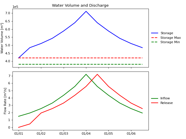
Extracting Results
The results from the run are found in output\timeseries_export.csv. Any
CSV-reading software can import it. Here we used matplotlib to generate this plot.
(Source code, svg, png)

Observations
This plot shows that the operator is not able to keep the water level within the bounds over the entire time horizon. They may need to increase the controller timestep, use a more complete PID controller, or use model predictive control such as the RTC-Tools optimization library to get the results they want.