Filling a Reservoir
Overview
The purpose of this example is to understand the technical setup of an RTC-Tools model, how to run the model, and how to interpret the results.
The scenario is the following: A reservoir operator is trying to fill a reservoir. They are given a six-day forecast of inflows given in 12-hour increments. The operator wants to save as much of the inflows as possible, but does not want to end up with too much water at the end of the six days. They have chosen to use RTC-Tools to calculate how much water to release and when to release it.
If you installed using source, the library and examples directory are available in the git repositories. If you installed using pip directly, you first need to download/copy the examples and libraries to a convenient location. See Downloading and running examples and Copying Modelica libraries for detailed instructions.
The folder <examples directory>\basic contains a complete RTC-Tools
optimization problem. An RTC-Tools directory has the following structure:
input: This folder contains the model input data. These are several files in comma separated value format,csv.model: This folder contains the Modelica model. The Modelica model contains the physics of the RTC-Tools model.output: The folder where the output is saved in the filetimeseries_export.csv.src: This folder contains a Python file. This file contains the configuration of the model and is used to run the model .
The Model
The first step is to develop a physical model of the system. The model can be viewed and edited using the OpenModelica Connection Editor (OMEdit) program. For how to download and start up OMEdit, see Getting OMEdit.
Load the Deltares library into OMEdit
Using the menu bar: File -> Open Model/Library File(s)
Select
<library directory>\Deltares\package.mo
Load the example model into OMEdit
Using the menu bar: File -> Open Model/Library File(s)
Select
<examples directory>\basic\model\Example.mo
Once loaded, we have an OpenModelica Connection Editor window that looks like this:
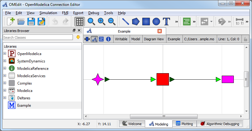
The model Example.mo represents a simple system with the following
elements:
a reservoir, modeled as storage element
Deltares.ChannelFlow.SimpleRouting.Storage.Storage,an inflow boundary condition
Deltares.ChannelFlow.SimpleRouting.BoundaryConditions.Inflow,an outfall boundary condition
Deltares.ChannelFlow.SimpleRouting.BoundaryConditions.Terminal,connectors (black lines) connecting the elements.
You can use the mouse-over feature help to identify the predefined models from the Deltares library. You can also drag the elements around- the connectors will move with the elements. Adding new elements is easy- just drag them in from the Deltares Library on the sidebar. Connecting the elements is just as easy- click and drag between the ports on the elements.
In text mode, the Modelica model looks as follows (with annotation statements removed):
 1model Example
 2  Deltares.ChannelFlow.SimpleRouting.BoundaryConditions.Inflow inflow;
 3  Deltares.ChannelFlow.SimpleRouting.Storage.Storage storage(V(nominal=4e5, min=2e5, max=6e5));
 4  Deltares.ChannelFlow.SimpleRouting.BoundaryConditions.Terminal outfall;
 5  input Modelica.SIunits.VolumeFlowRate Q_in(fixed = true);
 6  input Modelica.SIunits.VolumeFlowRate Q_release(fixed = false, min = 0.0, max = 6.5);
 7  output Modelica.SIunits.Volume V_storage;
 8equation
 9  connect(inflow.QOut, storage.QIn);
10  connect(storage.QOut, outfall.QIn);
11  storage.Q_release = Q_release;
12  inflow.Q = Q_in;
13  V_storage = storage.V;
14end Example;
The three water system elements (storage, inflow, and outfall) appear under
the model Example statement. The equation part connects these three
elements with the help of connections. Note that storage extends the partial
model QSISO which contains the connectors QIn and QOut.
With QSISO, storage can be connected on two sides. The storage
element also has a variable Q_release, which is the decision variable the
operator controls.
OpenModelica Connection Editor will automatically generate the element and
connector entries in the text text file. Defining inputs and outputs requires
editing the text file directly. Relationships between the inputs and outputs and
the library elements must also be defined in the equation section.
In addition to elements, the input variables Q_in and Q_release are also
defined. Q_in is determined by the forecast and the operator cannot control
it, so we set Q_in(fixed = true). The actual values of Q_in are stored
in timeseries_import.csv. In the equation section, equations are defined
to relate the inputs to the appropriate water system elements.
Because we want to view the water volume in the storage element in the output
file, we also define an output variable V_storage.
There is a subtle difference between these quantities: V_storage at time t holds
the volume of water in storage at that specific point in time. On the other hand,
Q_in and Q_release are aggregated measures: at time, t, their value
represents the total flow between time t-1 and t.
The Optimization Problem
The python script is created and edited in a text editor. In general, the python script consists of the following blocks:
Import of packages
Definition of the optimization problem class
Constructor
Objective function
Definition of constraints
Any additional configuration
A run statement
Importing Packages
Packages are imported using from ... import ... at the top of the file. In
our script, we import the classes we want the class to inherit, the
package run_optimization_problem form the rtctools.util package, and
any extra packages we want to use. For this example, the import block looks
like:
1from rtctools.optimization.collocated_integrated_optimization_problem import (
2    CollocatedIntegratedOptimizationProblem,
3)
4from rtctools.optimization.csv_mixin import CSVMixin
5from rtctools.optimization.modelica_mixin import ModelicaMixin
Optimization Problem
The next step is to define the optimization problem class. We construct the class by declaring the class and inheriting the desired parent classes. The parent classes each perform different tasks related to importing and exporting data and solving the optimization problem. Each imported class makes a set of methods available to the our optimization class.
9class Example(CSVMixin, ModelicaMixin, CollocatedIntegratedOptimizationProblem):
Next, we define an objective function. This is a class method that returns the value that needs to be minimized.
14    def objective(self, ensemble_member):
15        # Minimize water pumped. The total water pumped is the integral of the
16        # water pumped from the starting time until the stoping time. In
17        # practice, self.integral() is a summation of all the discrete states.
18        return self.integral("Q_release", ensemble_member=ensemble_member)
Constraints can be declared by declaring the path_constraints() method. Path
constraints are constraints that are applied every timestep. To set a constraint
at an individual timestep, we could define it inside the constraints() method.
Other parent classes also declare this method, so we call the super() method
so that we don’t overwrite their behaviour.
20    def path_constraints(self, ensemble_member):
21        # Call super() class to not overwrite default behaviour
22        constraints = super().path_constraints(ensemble_member)
23        # Constrain the volume of storage between 380000 and 420000 m^3
24        constraints.append((self.state("storage.V"), 380000, 420000))
25        return constraints
Run the Optimization Problem
To make our script run, at the bottom of our file we just have to call
the run_optimization_problem() method we imported on the optimization
problem class we just created.
29run_optimization_problem(Example)
The Whole Script
All together, the whole example script is as follows:
 1from rtctools.optimization.collocated_integrated_optimization_problem import (
 2    CollocatedIntegratedOptimizationProblem,
 3)
 4from rtctools.optimization.csv_mixin import CSVMixin
 5from rtctools.optimization.modelica_mixin import ModelicaMixin
 6from rtctools.util import run_optimization_problem
 7
 8
 9class Example(CSVMixin, ModelicaMixin, CollocatedIntegratedOptimizationProblem):
10    """
11    A basic example for introducing users to RTC-Tools 2
12    """
13
14    def objective(self, ensemble_member):
15        # Minimize water pumped. The total water pumped is the integral of the
16        # water pumped from the starting time until the stoping time. In
17        # practice, self.integral() is a summation of all the discrete states.
18        return self.integral("Q_release", ensemble_member=ensemble_member)
19
20    def path_constraints(self, ensemble_member):
21        # Call super() class to not overwrite default behaviour
22        constraints = super().path_constraints(ensemble_member)
23        # Constrain the volume of storage between 380000 and 420000 m^3
24        constraints.append((self.state("storage.V"), 380000, 420000))
25        return constraints
26
27
28# Run
29run_optimization_problem(Example)
Running RTC-Tools
To run this basic example in RTC-Tools, navigate to the basic example src
directory in the RTC-Tools shell and run the example using python
example.py. For more details about using RTC-Tools, see
Running RTC-Tools.
Extracting Results
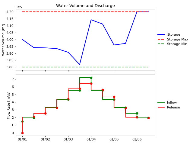
The results from the run are found in output\timeseries_export.csv. Any
CSV-reading software can import it, but this is what the results look like when
plotted with the python library matplotlib:
(Source code, svg, png)

This plot shows that the operator is able to keep the water level within the bounds over the entire time horizon and end with a full reservoir.
Feel free to experiment with this example. See what happens if you change the
max of Q_release (in the Modelica file) or if you make the objective
function negative (in the python script).